Похоже, вы используете блокировщик рекламы. Наш сайт существует и развивается
только за счет дохода от рекламы.
Пожалуйста, добавьте нас в исключения блокировщика.


на главную
Как найти координаты точки
Поддержать сайт![]()
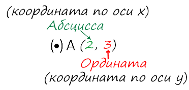
Каждой точке координатной плоскости соответствуют две координаты.
Координаты точки на плоскости — это пара чисел, в которой на
первом месте стоит
абсцисса, а на
втором —
ордината точки.
Рассмотрим как в системе координат (на координатной плоскости):
- находить координаты точки;
- найти положение точки.
Чтобы найти координаты точки на плоскости, нужно опустить из этой точки
перпендикуляры на оси координат.
Точка пересечения с осью «x» называется абсциссой точки «А»,
а с осью y называется ординатой точки «А».
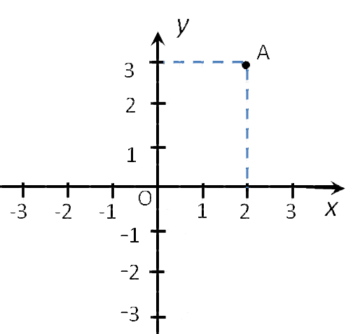
Обозначают координаты точки, как указано выше (·) A (2; 3).
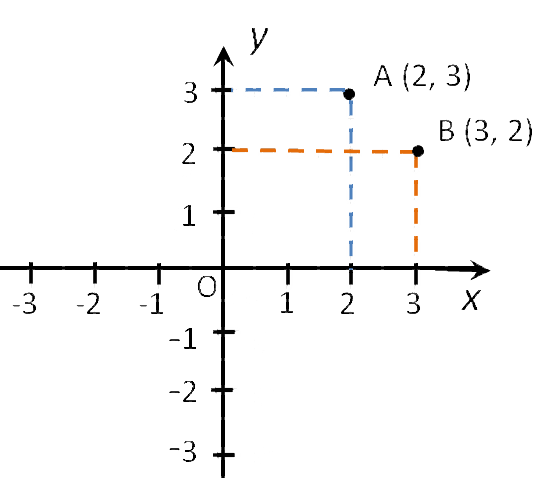
Пример (·) A (2; 3) и (·) B (3; 2).
Запомните!
![]()
На первом месте записывают абсциссу (координату по оси «x»), а на втором —
ординату (координату по оси «y») точки.
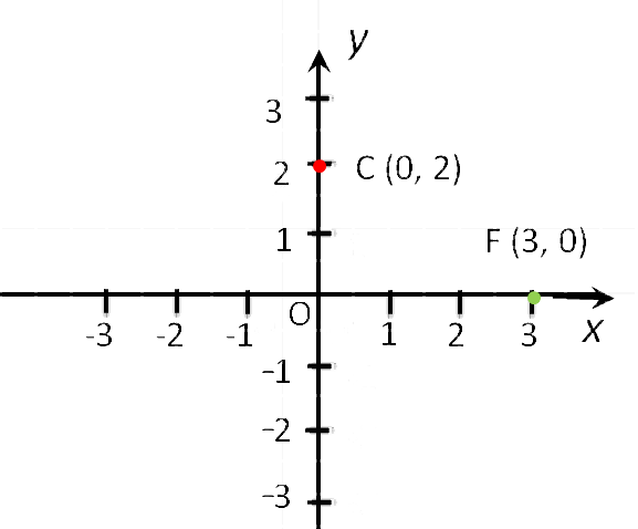
Особые случаи расположения точек
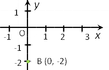
- Если точка лежит на оси «Oy»,
то её абсцисса равна 0. Например,
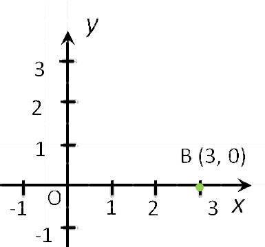
точка С (0, 2). - Если точка лежит на оси «Ox», то её ордината равна 0.
Например,
точка F (3, 0). - Начало координат — точка O имеет координаты, равные нулю O (0,0).

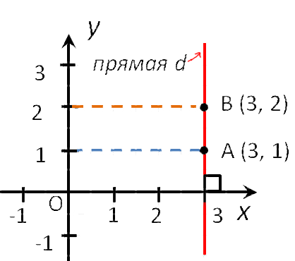
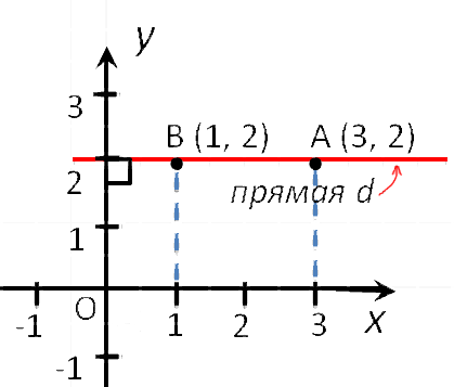
- Точки любой прямой перпендикулярной оси абсцисс, имеют одинаковые абсциссы.
- Точки любой прямой перпендикулярной оси ординат, имеют одинаковые ординаты.
- Координаты любой точки, лежащей на оси абсцисс имеют вид (x, 0).
- Координаты любой точки, лежащей на оси ординат имеют вид (0, y).
Как найти положение точки по её координатам
Найти точку в системе координат можно двумя способами.
Первый способ
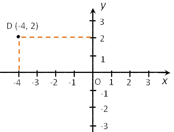
Чтобы определить положение точки по её координатам,
например, точки D (−4 , 2), надо:
- Отметить на оси «Ox», точку с координатой
«−4», и провести через неё прямую перпендикулярную оси «Ox». - Отметить на оси «Oy»,
точку с координатой 2, и провести через неё прямую перпендикулярную
оси «Oy». - Точка пересечения перпендикуляров (·) D — искомая точка.
У неё абсцисса равна «−4», а ордината равна 2.
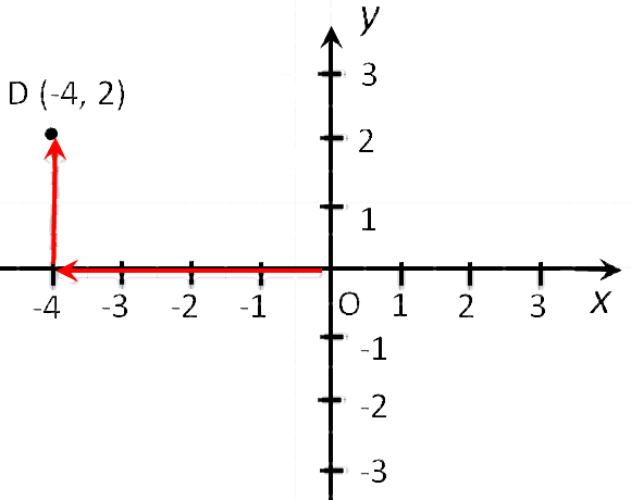
Второй способ
Чтобы найти точку D (−4 , 2) надо:
- Сместиться по оси «x» влево на
4 единицы, так как у нас
перед 4
стоит «−». - Подняться из этой точки параллельно оси y вверх на 2 единицы, так
как у нас перед 2 стоит «+».
Чтобы быстрее и удобнее было находить координаты точек или строить точки по координатам на
листе формата A4 в клеточку, можно скачать и использовать
готовую систему координат на нашем сайте.

Illustration of a Cartesian coordinate plane. Four points are marked and labeled with their coordinates: (2, 3) in green, (−3, 1) in red, (−1.5, −2.5) in blue, and the origin (0, 0) in purple.
A Cartesian coordinate system (, ) in a plane is a coordinate system that specifies each point uniquely by a pair of numerical coordinates, which are the signed distances to the point from two fixed perpendicular oriented lines, measured in the same unit of length. Each reference coordinate line is called a coordinate axis or just axis (plural axes) of the system, and the point where they meet is its origin, at ordered pair (0, 0). The coordinates can also be defined as the positions of the perpendicular projections of the point onto the two axes, expressed as signed distances from the origin.
One can use the same principle to specify the position of any point in three-dimensional space by three Cartesian coordinates, its signed distances to three mutually perpendicular planes (or, equivalently, by its perpendicular projection onto three mutually perpendicular lines). In general, n Cartesian coordinates (an element of real n-space) specify the point in an n-dimensional Euclidean space for any dimension n. These coordinates are equal, up to sign, to distances from the point to n mutually perpendicular hyperplanes.
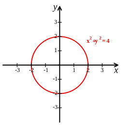
Cartesian coordinate system with a circle of radius 2 centered at the origin marked in red. The equation of a circle is (x − a)2 + (y − b)2 = r2 where a and b are the coordinates of the center (a, b) and r is the radius.
Cartesian coordinates are named for René Descartes whose invention of them in the 17th century revolutionized mathematics by providing the first systematic link between Euclidean geometry and algebra. Using the Cartesian coordinate system, geometric shapes (such as curves) can be described by Cartesian equations: algebraic equations involving the coordinates of the points lying on the shape. For example, a circle of radius 2, centered at the origin of the plane, may be described as the set of all points whose coordinates x and y satisfy the equation x2 + y2 = 4.
Cartesian coordinates are the foundation of analytic geometry, and provide enlightening geometric interpretations for many other branches of mathematics, such as linear algebra, complex analysis, differential geometry, multivariate calculus, group theory and more. A familiar example is the concept of the graph of a function. Cartesian coordinates are also essential tools for most applied disciplines that deal with geometry, including astronomy, physics, engineering and many more. They are the most common coordinate system used in computer graphics, computer-aided geometric design and other geometry-related data processing.
History[edit]
The adjective Cartesian refers to the French mathematician and philosopher René Descartes, who published this idea in 1637 while he was resident in the Netherlands. It was independently discovered by Pierre de Fermat, who also worked in three dimensions, although Fermat did not publish the discovery.[1] The French cleric Nicole Oresme used constructions similar to Cartesian coordinates well before the time of Descartes and Fermat.[2]
Both Descartes and Fermat used a single axis in their treatments and have a variable length measured in reference to this axis. The concept of using a pair of axes was introduced later, after Descartes’ La Géométrie was translated into Latin in 1649 by Frans van Schooten and his students. These commentators introduced several concepts while trying to clarify the ideas contained in Descartes’s work.[3]
The development of the Cartesian coordinate system would play a fundamental role in the development of the calculus by Isaac Newton and Gottfried Wilhelm Leibniz.[4] The two-coordinate description of the plane was later generalized into the concept of vector spaces.[5]
Many other coordinate systems have been developed since Descartes, such as the polar coordinates for the plane, and the spherical and cylindrical coordinates for three-dimensional space.
Description[edit]
One dimension [edit]
Choosing a Cartesian coordinate system for a one-dimensional space—that is, for a straight line—involves choosing a point O of the line (the origin), a unit of length, and an orientation for the line. An orientation chooses which of the two half-lines determined by O is the positive and which is negative; we then say that the line «is oriented» (or «points») from the negative half towards the positive half. Then each point P of the line can be specified by its distance from O, taken with a + or − sign depending on which half-line contains P.
A line with a chosen Cartesian system is called a number line. Every real number has a unique location on the line. Conversely, every point on the line can be interpreted as a number in an ordered continuum such as the real numbers.
Two dimensions [edit]
A Cartesian coordinate system in two dimensions (also called a rectangular coordinate system or an orthogonal coordinate system[6]) is defined by an ordered pair of perpendicular lines (axes), a single unit of length for both axes, and an orientation for each axis. The point where the axes meet is taken as the origin for both, thus turning each axis into a number line. For any point P, a line is drawn through P perpendicular to each axis, and the position where it meets the axis is interpreted as a number. The two numbers, in that chosen order, are the Cartesian coordinates of P. The reverse construction allows one to determine the point P given its coordinates.
The first and second coordinates are called the abscissa and the ordinate of P, respectively; and the point where the axes meet is called the origin of the coordinate system. The coordinates are usually written as two numbers in parentheses, in that order, separated by a comma, as in (3, −10.5). Thus the origin has coordinates (0, 0), and the points on the positive half-axes, one unit away from the origin, have coordinates (1, 0) and (0, 1).
In mathematics, physics, and engineering, the first axis is usually defined or depicted as horizontal and oriented to the right, and the second axis is vertical and oriented upwards. (However, in some computer graphics contexts, the ordinate axis may be oriented downwards.) The origin is often labeled O, and the two coordinates are often denoted by the letters X and Y, or x and y. The axes may then be referred to as the X-axis and Y-axis. The choices of letters come from the original convention, which is to use the latter part of the alphabet to indicate unknown values. The first part of the alphabet was used to designate known values.
A Euclidean plane with a chosen Cartesian coordinate system is called a Cartesian plane. In a Cartesian plane one can define canonical representatives of certain geometric figures, such as the unit circle (with radius equal to the length unit, and center at the origin), the unit square (whose diagonal has endpoints at (0, 0) and (1, 1)), the unit hyperbola, and so on.
The two axes divide the plane into four right angles, called quadrants. The quadrants may be named or numbered in various ways, but the quadrant where all coordinates are positive is usually called the first quadrant.
If the coordinates of a point are (x, y), then its distances from the X-axis and from the Y-axis are |y| and |x|, respectively; where | · | denotes the absolute value of a number.
Three dimensions [edit]
A three dimensional Cartesian coordinate system, with origin O and axis lines X, Y and Z, oriented as shown by the arrows. The tick marks on the axes are one length unit apart. The black dot shows the point with coordinates x = 2, y = 3, and z = 4, or (2, 3, 4).
A Cartesian coordinate system for a three-dimensional space consists of an ordered triplet of lines (the axes) that go through a common point (the origin), and are pair-wise perpendicular; an orientation for each axis; and a single unit of length for all three axes. As in the two-dimensional case, each axis becomes a number line. For any point P of space, one considers a hyperplane through P perpendicular to each coordinate axis, and interprets the point where that hyperplane cuts the axis as a number. The Cartesian coordinates of P are those three numbers, in the chosen order. The reverse construction determines the point P given its three coordinates.
Alternatively, each coordinate of a point P can be taken as the distance from P to the hyperplane defined by the other two axes, with the sign determined by the orientation of the corresponding axis.
Each pair of axes defines a coordinate hyperplane. These hyperplanes divide space into eight octants. The octants are:

The coordinates are usually written as three numbers (or algebraic formulas) surrounded by parentheses and separated by commas, as in (3, −2.5, 1) or (t, u + v, π/2). Thus, the origin has coordinates (0, 0, 0), and the unit points on the three axes are (1, 0, 0), (0, 1, 0), and (0, 0, 1).
There are no standard names for the coordinates in the three axes (however, the terms abscissa, ordinate and applicate are sometimes used). The coordinates are often denoted by the letters X, Y, and Z, or x, y, and z. The axes may then be referred to as the X-axis, Y-axis, and Z-axis, respectively. Then the coordinate hyperplanes can be referred to as the XY-plane, YZ-plane, and XZ-plane.
In mathematics, physics, and engineering contexts, the first two axes are often defined or depicted as horizontal, with the third axis pointing up. In that case the third coordinate may be called height or altitude. The orientation is usually chosen so that the 90 degree angle from the first axis to the second axis looks counter-clockwise when seen from the point (0, 0, 1); a convention that is commonly called the right hand rule.

The coordinate surfaces of the Cartesian coordinates (x, y, z). The z-axis is vertical and the x-axis is highlighted in green. Thus, the red hyperplane shows the points with x = 1, the blue hyperplane shows the points with z = 1, and the yellow hyperplane shows the points with y = −1. The three surfaces intersect at the point P (shown as a black sphere) with the Cartesian coordinates (1, −1, 1).
Higher dimensions[edit]
Since Cartesian coordinates are unique and non-ambiguous, the points of a Cartesian plane can be identified with pairs of real numbers; that is, with the Cartesian product  , where
  is the set of all real numbers. In the same way, the points in any Euclidean space of dimension n be identified with the tuples (lists) of n real numbers; that is, with the Cartesian product
  .
.
Generalizations[edit]
The concept of Cartesian coordinates generalizes to allow axes that are not perpendicular to each other, and/or different units along each axis. In that case, each coordinate is obtained by projecting the point onto one axis along a direction that is parallel to the other axis (or, in general, to the hyperplane defined by all the other axes). In such an oblique coordinate system the computations of distances and angles must be modified from that in standard Cartesian systems, and many standard formulas (such as the Pythagorean formula for the distance) do not hold (see affine plane).
Notations and conventions[edit]
The Cartesian coordinates of a point are usually written in parentheses and separated by commas, as in (10, 5) or (3, 5, 7). The origin is often labelled with the capital letter O. In analytic geometry, unknown or generic coordinates are often denoted by the letters (x, y) in the plane, and (x, y, z) in three-dimensional space. This custom comes from a convention of algebra, which uses letters near the end of the alphabet for unknown values (such as the coordinates of points in many geometric problems), and letters near the beginning for given quantities.
These conventional names are often used in other domains, such as physics and engineering, although other letters may be used. For example, in a graph showing how a pressure varies with time, the graph coordinates may be denoted p and t. Each axis is usually named after the coordinate which is measured along it; so one says the x-axis, the y-axis, the t-axis, etc.
Another common convention for coordinate naming is to use subscripts, as (x1, x2, …, xn) for the n coordinates in an n-dimensional space, especially when n is greater than 3 or unspecified. Some authors prefer the numbering (x0, x1, …, xn−1). These notations are especially advantageous in computer programming: by storing the coordinates of a point as an array, instead of a record, the subscript can serve to index the coordinates.
In mathematical illustrations of two-dimensional Cartesian systems, the first coordinate (traditionally called the abscissa) is measured along a horizontal axis, oriented from left to right. The second coordinate (the ordinate) is then measured along a vertical axis, usually oriented from bottom to top. Young children learning the Cartesian system, commonly learn the order to read the values before cementing the x-, y-, and z-axis concepts, by starting with 2D mnemonics (for example, ‘Walk along the hall then up the stairs’ akin to straight across the x-axis then up vertically along the y-axis).[7]
Computer graphics and image processing, however, often use a coordinate system with the y-axis oriented downwards on the computer display. This convention developed in the 1960s (or earlier) from the way that images were originally stored in display buffers.
For three-dimensional systems, a convention is to portray the xy-plane horizontally, with the z-axis added to represent height (positive up). Furthermore, there is a convention to orient the x-axis toward the viewer, biased either to the right or left. If a diagram (3D projection or 2D perspective drawing) shows the x— and y-axis horizontally and vertically, respectively, then the z-axis should be shown pointing «out of the page» towards the viewer or camera. In such a 2D diagram of a 3D coordinate system, the z-axis would appear as a line or ray pointing down and to the left or down and to the right, depending on the presumed viewer or camera perspective. In any diagram or display, the orientation of the three axes, as a whole, is arbitrary. However, the orientation of the axes relative to each other should always comply with the right-hand rule, unless specifically stated otherwise. All laws of physics and math assume this right-handedness, which ensures consistency.
For 3D diagrams, the names «abscissa» and «ordinate» are rarely used for x and y, respectively. When they are, the z-coordinate is sometimes called the applicate. The words abscissa, ordinate and applicate are sometimes used to refer to coordinate axes rather than the coordinate values.[6]
Quadrants and octants[edit]

The four quadrants of a Cartesian coordinate system
The axes of a two-dimensional Cartesian system divide the plane into four infinite regions, called quadrants,[6] each bounded by two half-axes. These are often numbered from 1st to 4th and denoted by Roman numerals: I (where the coordinates both have positive signs), II (where the abscissa is negative − and the ordinate is positive +), III (where both the abscissa and the ordinate are −), and IV (abscissa +, ordinate −). When the axes are drawn according to the mathematical custom, the numbering goes counter-clockwise starting from the upper right («north-east») quadrant.
Similarly, a three-dimensional Cartesian system defines a division of space into eight regions or octants,[6] according to the signs of the coordinates of the points. The convention used for naming a specific octant is to list its signs; for example, (+ + +) or (− + −). The generalization of the quadrant and octant to an arbitrary number of dimensions is the orthant, and a similar naming system applies.
Cartesian formulae for the plane[edit]
Distance between two points[edit]
The Euclidean distance between two points of the plane with Cartesian coordinates  and
and  is
is

This is the Cartesian version of Pythagoras’s theorem. In three-dimensional space, the distance between points  and
and  is
is

which can be obtained by two consecutive applications of Pythagoras’ theorem.[8]
Euclidean transformations[edit]
The Euclidean transformations or Euclidean motions are the (bijective) mappings of points of the Euclidean plane to themselves which preserve distances between points. There are four types of these mappings (also called isometries): translations, rotations, reflections and glide reflections.[9]
Translation[edit]
Translating a set of points of the plane, preserving the distances and directions between them, is equivalent to adding a fixed pair of numbers (a, b) to the Cartesian coordinates of every point in the set. That is, if the original coordinates of a point are (x, y), after the translation they will be

Rotation[edit]
To rotate a figure counterclockwise around the origin by some angle  is equivalent to replacing every point with coordinates (x,y) by the point with coordinates (x’,y’), where

Thus:

Reflection[edit]
If (x, y) are the Cartesian coordinates of a point, then (−x, y) are the coordinates of its reflection across the second coordinate axis (the y-axis), as if that line were a mirror. Likewise, (x, −y) are the coordinates of its reflection across the first coordinate axis (the x-axis). In more generality, reflection across a line through the origin making an angle with the x-axis, is equivalent to replacing every point with coordinates (x, y) by the point with coordinates (x′,y′), where

Thus:

Glide reflection[edit]
A glide reflection is the composition of a reflection across a line followed by a translation in the direction of that line. It can be seen that the order of these operations does not matter (the translation can come first, followed by the reflection).
General matrix form of the transformations[edit]
All affine transformations of the plane can be described in a uniform way by using matrices. For this purpose the coordinates  of a point are commonly represented as the column matrix
  The result
  of applying an affine transformation to a point is given by the formula

where

is a 2×2 matrix and  is a column matrix.[10] That is,

Among the affine transformations, the Euclidean transformations are characterized by the fact that the matrix  is orthogonal; that is, its columns are orthogonal vectors of Euclidean norm one, or, explicitly,

and

This is equivalent to saying that A times its transpose is the identity matrix. If these conditions do not hold, the formula describes a more general affine transformation.
The transformation is a translation if and only if A is the identity matrix. The transformation is a rotation around some point if and only if A is a rotation matrix, meaning that it is orthogonal and

A reflection or glide reflection is obtained when,

Assuming that translations are not used (that is,  ) transformations can be composed by simply multiplying the associated transformation matrices. In the general case, it is useful to use the augmented matrix of the transformation; that is, to rewrite the transformation formula

where

With this trick, the composition of affine transformations is obtained by multiplying the augmented matrices.
Affine transformation[edit]
![]()
Effect of applying various 2D affine transformation matrices on a unit square (reflections are special cases of scaling)
Affine transformations of the Euclidean plane are transformations that map lines to lines, but may change distances and angles. As said in the preceding section, they can be represented with augmented matrices:

The Euclidean transformations are the affine transformations such that the 2×2 matrix of the  is orthogonal.
The augmented matrix that represents the composition of two affine transformations is obtained by multiplying their augmented matrices.
Some affine transformations that are not Euclidean transformations have received specific names.
Scaling[edit]
An example of an affine transformation which is not Euclidean is given by scaling. To make a figure larger or smaller is equivalent to multiplying the Cartesian coordinates of every point by the same positive number m. If (x, y) are the coordinates of a point on the original figure, the corresponding point on the scaled figure has coordinates

If m is greater than 1, the figure becomes larger; if m is between 0 and 1, it becomes smaller.
Shearing[edit]
A shearing transformation will push the top of a square sideways to form a parallelogram. Horizontal shearing is defined by:

Shearing can also be applied vertically:

Orientation and handedness[edit]
In two dimensions[edit]

Fixing or choosing the x-axis determines the y-axis up to direction. Namely, the y-axis is necessarily the perpendicular to the x-axis through the point marked 0 on the x-axis. But there is a choice of which of the two half lines on the perpendicular to designate as positive and which as negative. Each of these two choices determines a different orientation (also called handedness) of the Cartesian plane.
The usual way of orienting the plane, with the positive x-axis pointing right and the positive y-axis pointing up (and the x-axis being the «first» and the y-axis the «second» axis), is considered the positive or standard orientation, also called the right-handed orientation.
A commonly used mnemonic for defining the positive orientation is the right-hand rule. Placing a somewhat closed right hand on the plane with the thumb pointing up, the fingers point from the x-axis to the y-axis, in a positively oriented coordinate system.
The other way of orienting the plane is following the left hand rule, placing the left hand on the plane with the thumb pointing up.
When pointing the thumb away from the origin along an axis towards positive, the curvature of the fingers indicates a positive rotation along that axis.
Regardless of the rule used to orient the plane, rotating the coordinate system will preserve the orientation. Switching any one axis will reverse the orientation, but switching both will leave the orientation unchanged.
In three dimensions[edit]

Fig. 7 – The left-handed orientation is shown on the left, and the right-handed on the right.
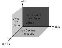
Fig. 8 – The right-handed Cartesian coordinate system indicating the coordinate planes.
Once the x— and y-axes are specified, they determine the line along which the z-axis should lie, but there are two possible orientation for this line. The two possible coordinate systems which result are called ‘right-handed’ and ‘left-handed’. The standard orientation, where the xy-plane is horizontal and the z-axis points up (and the x— and the y-axis form a positively oriented two-dimensional coordinate system in the xy-plane if observed from above the xy-plane) is called right-handed or positive.

3D Cartesian coordinate handedness
The name derives from the right-hand rule. If the index finger of the right hand is pointed forward, the middle finger bent inward at a right angle to it, and the thumb placed at a right angle to both, the three fingers indicate the relative orientation of the x-, y-, and z-axes in a right-handed system. The thumb indicates the x-axis, the index finger the y-axis and the middle finger the z-axis. Conversely, if the same is done with the left hand, a left-handed system results.
Figure 7 depicts a left and a right-handed coordinate system. Because a three-dimensional object is represented on the two-dimensional screen, distortion and ambiguity result. The axis pointing downward (and to the right) is also meant to point towards the observer, whereas the «middle»-axis is meant to point away from the observer. The red circle is parallel to the horizontal xy-plane and indicates rotation from the x-axis to the y-axis (in both cases). Hence the red arrow passes in front of the z-axis.
Figure 8 is another attempt at depicting a right-handed coordinate system. Again, there is an ambiguity caused by projecting the three-dimensional coordinate system into the plane. Many observers see Figure 8 as «flipping in and out» between a convex cube and a concave «corner». This corresponds to the two possible orientations of the space. Seeing the figure as convex gives a left-handed coordinate system. Thus the «correct» way to view Figure 8 is to imagine the x-axis as pointing towards the observer and thus seeing a concave corner.
Representing a vector in the standard basis[edit]
A point in space in a Cartesian coordinate system may also be represented by a position vector, which can be thought of as an arrow pointing from the origin of the coordinate system to the point.[11] If the coordinates represent spatial positions (displacements), it is common to represent the vector from the origin to the point of interest as  . In two dimensions, the vector from the origin to the point with Cartesian coordinates (x, y) can be written as:

where  and
and  are unit vectors in the direction of the x-axis and y-axis respectively, generally referred to as the standard basis (in some application areas these may also be referred to as versors). Similarly, in three dimensions, the vector from the origin to the point with Cartesian coordinates
  can be written as:[12]

where 
 and
and 
There is no natural interpretation of multiplying vectors to obtain another vector that works in all dimensions, however there is a way to use complex numbers to provide such a multiplication. In a two-dimensional cartesian plane, identify the point with coordinates (x, y) with the complex number z = x + iy. Here, i is the imaginary unit and is identified with the point with coordinates (0, 1), so it is not the unit vector in the direction of the x-axis. Since the complex numbers can be multiplied giving another complex number, this identification provides a means to «multiply» vectors. In a three-dimensional cartesian space a similar identification can be made with a subset of the quaternions.
Applications[edit]
Cartesian coordinates are an abstraction that have a multitude of possible applications in the real world. However, three constructive steps are involved in superimposing coordinates on a problem application.
- Units of distance must be decided defining the spatial size represented by the numbers used as coordinates.
- An origin must be assigned to a specific spatial location or landmark, and
- the orientation of the axes must be defined using available directional cues for all but one axis.
Consider as an example superimposing 3D Cartesian coordinates over all points on the Earth (that is, geospatial 3D). Kilometers are a good choice of units, since the original definition of the kilometer was geospatial, with 10,000 km equaling the surface distance from the equator to the North Pole. Based on symmetry, the gravitational center of the Earth suggests a natural placement of the origin (which can be sensed via satellite orbits). The axis of Earth’s rotation provides a natural orientation for the X, Y, and Z axes, strongly associated with «up vs. down», so positive Z can adopt the direction from the geocenter to the North Pole. A location on the equator is needed to define the X-axis, and the prime meridian stands out as a reference orientation, so the X-axis takes the orientation from the geocenter out to 0 degrees longitude, 0 degrees latitude. Note that with three dimensions, and two perpendicular axes orientations pinned down for X and Z, the Y-axis is determined by the first two choices. In order to obey the right-hand rule, the Y-axis must point out from the geocenter to 90 degrees longitude, 0 degrees latitude. From a longitude of −73.985656 degrees, a latitude 40.748433 degrees, and Earth radius of 40,000/2π km, and transforming from spherical to Cartesian coordinates, one can estimate the geocentric coordinates of the Empire State Building, (x, y, z) = (1,330.53 km, 4,635.75 km, 4,155.46 km). GPS navigation relies on such geocentric coordinates.
In engineering projects, agreement on the definition of coordinates is a crucial foundation. One cannot assume that coordinates come predefined for a novel application, so knowledge of how to erect a coordinate system where there previously was no such coordinate system is essential to applying René Descartes’ thinking.
While spatial applications employ identical units along all axes, in business and scientific applications, each axis may have different units of measurement associated with it (such as kilograms, seconds, pounds, etc.). Although four- and higher-dimensional spaces are difficult to visualize, the algebra of Cartesian coordinates can be extended relatively easily to four or more variables, so that certain calculations involving many variables can be done. (This sort of algebraic extension is what is used to define the geometry of higher-dimensional spaces.) Conversely, it is often helpful to use the geometry of Cartesian coordinates in two or three dimensions to visualize algebraic relationships between two or three of many non-spatial variables.
The graph of a function or relation is the set of all points satisfying that function or relation. For a function of one variable, f, the set of all points (x, y), where y = f(x) is the graph of the function f. For a function g of two variables, the set of all points (x, y, z), where z = g(x, y) is the graph of the function g. A sketch of the graph of such a function or relation would consist of all the salient parts of the function or relation which would include its relative extrema, its concavity and points of inflection, any points of discontinuity and its end behavior. All of these terms are more fully defined in calculus. Such graphs are useful in calculus to understand the nature and behavior of a function or relation.
See also[edit]
- Horizontal and vertical
- Jones diagram, which plots four variables rather than two
- Orthogonal coordinates
- Polar coordinate system
- Regular grid
- Spherical coordinate system
References[edit]
- ^ Bix, Robert A.; D’Souza, Harry J. «Analytic geometry». Encyclopædia Britannica. Retrieved 6 August 2017.
- ^ Kent, Alexander J.; Vujakovic, Peter (4 October 2017). The Routledge Handbook of Mapping and Cartography. Routledge. ISBN 9781317568216.
- ^ Burton 2011, p. 374.
- ^ A Tour of the Calculus, David Berlinski.
- ^ Axler, Sheldon (2015). Linear Algebra Done Right – Springer. Undergraduate Texts in Mathematics. p. 1. doi:10.1007/978-3-319-11080-6. ISBN 978-3-319-11079-0.
- ^ a b c d «Cartesian orthogonal coordinate system». Encyclopedia of Mathematics. Retrieved 6 August 2017.
- ^ «Charts and Graphs: Choosing the Right Format». mindtools.com. Retrieved 29 August 2017.
- ^ Hughes-Hallett, Deborah; McCallum, William G.; Gleason, Andrew M. (2013). Calculus : Single and Multivariable (6 ed.). John wiley. ISBN 978-0470-88861-2.
- ^ Smart 1998, Chap. 2
- ^ Brannan, Esplen & Gray 1998, pg. 49
- ^ Brannan, Esplen & Gray 1998, Appendix 2, pp. 377–382
- ^ David J. Griffiths (1999). Introduction to Electrodynamics. Prentice Hall. ISBN 978-0-13-805326-0.
Sources[edit]
- Brannan, David A.; Esplen, Matthew F.; Gray, Jeremy J. (1998), Geometry, Cambridge: Cambridge University Press, ISBN 978-0-521-59787-6
- Burton, David M. (2011), The History of Mathematics/An Introduction (7th ed.), New York: McGraw-Hill, ISBN 978-0-07-338315-6
- Smart, James R. (1998), Modern Geometries (5th ed.), Pacific Grove: Brooks/Cole, ISBN 978-0-534-35188-5
Further reading[edit]
- Descartes, René (2001). Discourse on Method, Optics, Geometry, and Meteorology. Translated by Paul J. Oscamp (Revised ed.). Indianapolis, IN: Hackett Publishing. ISBN 978-0-87220-567-3. OCLC 488633510.
- Korn GA, Korn TM (1961). Mathematical Handbook for Scientists and Engineers (1st ed.). New York: McGraw-Hill. pp. 55–79. LCCN 59-14456. OCLC 19959906.
- Margenau H, Murphy GM (1956). The Mathematics of Physics and Chemistry. New York: D. van Nostrand. LCCN 55-10911.
- Moon P, Spencer DE (1988). «Rectangular Coordinates (x, y, z)». Field Theory Handbook, Including Coordinate Systems, Differential Equations, and Their Solutions (corrected 2nd, 3rd print ed.). New York: Springer-Verlag. pp. 9–11 (Table 1.01). ISBN 978-0-387-18430-2.
- Morse PM, Feshbach H (1953). Methods of Theoretical Physics, Part I. New York: McGraw-Hill. ISBN 978-0-07-043316-8. LCCN 52-11515.
- Sauer R, Szabó I (1967). Mathematische Hilfsmittel des Ingenieurs. New York: Springer Verlag. LCCN 67-25285.
External links[edit]
- Cartesian Coordinate System
- MathWorld description of Cartesian coordinates
- Coordinate Converter – converts between polar, Cartesian and spherical coordinates
- Coordinates of a point Interactive tool to explore coordinates of a point
- open source JavaScript class for 2D/3D Cartesian coordinate system manipulation
Illustration of a Cartesian coordinate plane. Four points are marked and labeled with their coordinates: (2, 3) in green, (−3, 1) in red, (−1.5, −2.5) in blue, and the origin (0, 0) in purple.
A Cartesian coordinate system (, ) in a plane is a coordinate system that specifies each point uniquely by a pair of numerical coordinates, which are the signed distances to the point from two fixed perpendicular oriented lines, measured in the same unit of length. Each reference coordinate line is called a coordinate axis or just axis (plural axes) of the system, and the point where they meet is its origin, at ordered pair (0, 0). The coordinates can also be defined as the positions of the perpendicular projections of the point onto the two axes, expressed as signed distances from the origin.
One can use the same principle to specify the position of any point in three-dimensional space by three Cartesian coordinates, its signed distances to three mutually perpendicular planes (or, equivalently, by its perpendicular projection onto three mutually perpendicular lines). In general, n Cartesian coordinates (an element of real n-space) specify the point in an n-dimensional Euclidean space for any dimension n. These coordinates are equal, up to sign, to distances from the point to n mutually perpendicular hyperplanes.
Cartesian coordinate system with a circle of radius 2 centered at the origin marked in red. The equation of a circle is (x − a)2 + (y − b)2 = r2 where a and b are the coordinates of the center (a, b) and r is the radius.
Cartesian coordinates are named for René Descartes whose invention of them in the 17th century revolutionized mathematics by providing the first systematic link between Euclidean geometry and algebra. Using the Cartesian coordinate system, geometric shapes (such as curves) can be described by Cartesian equations: algebraic equations involving the coordinates of the points lying on the shape. For example, a circle of radius 2, centered at the origin of the plane, may be described as the set of all points whose coordinates x and y satisfy the equation x2 + y2 = 4.
Cartesian coordinates are the foundation of analytic geometry, and provide enlightening geometric interpretations for many other branches of mathematics, such as linear algebra, complex analysis, differential geometry, multivariate calculus, group theory and more. A familiar example is the concept of the graph of a function. Cartesian coordinates are also essential tools for most applied disciplines that deal with geometry, including astronomy, physics, engineering and many more. They are the most common coordinate system used in computer graphics, computer-aided geometric design and other geometry-related data processing.
History[edit]
The adjective Cartesian refers to the French mathematician and philosopher René Descartes, who published this idea in 1637 while he was resident in the Netherlands. It was independently discovered by Pierre de Fermat, who also worked in three dimensions, although Fermat did not publish the discovery.[1] The French cleric Nicole Oresme used constructions similar to Cartesian coordinates well before the time of Descartes and Fermat.[2]
Both Descartes and Fermat used a single axis in their treatments and have a variable length measured in reference to this axis. The concept of using a pair of axes was introduced later, after Descartes’ La Géométrie was translated into Latin in 1649 by Frans van Schooten and his students. These commentators introduced several concepts while trying to clarify the ideas contained in Descartes’s work.[3]
The development of the Cartesian coordinate system would play a fundamental role in the development of the calculus by Isaac Newton and Gottfried Wilhelm Leibniz.[4] The two-coordinate description of the plane was later generalized into the concept of vector spaces.[5]
Many other coordinate systems have been developed since Descartes, such as the polar coordinates for the plane, and the spherical and cylindrical coordinates for three-dimensional space.
Description[edit]
One dimension [edit]
Choosing a Cartesian coordinate system for a one-dimensional space—that is, for a straight line—involves choosing a point O of the line (the origin), a unit of length, and an orientation for the line. An orientation chooses which of the two half-lines determined by O is the positive and which is negative; we then say that the line «is oriented» (or «points») from the negative half towards the positive half. Then each point P of the line can be specified by its distance from O, taken with a + or − sign depending on which half-line contains P.
A line with a chosen Cartesian system is called a number line. Every real number has a unique location on the line. Conversely, every point on the line can be interpreted as a number in an ordered continuum such as the real numbers.
Two dimensions [edit]
A Cartesian coordinate system in two dimensions (also called a rectangular coordinate system or an orthogonal coordinate system[6]) is defined by an ordered pair of perpendicular lines (axes), a single unit of length for both axes, and an orientation for each axis. The point where the axes meet is taken as the origin for both, thus turning each axis into a number line. For any point P, a line is drawn through P perpendicular to each axis, and the position where it meets the axis is interpreted as a number. The two numbers, in that chosen order, are the Cartesian coordinates of P. The reverse construction allows one to determine the point P given its coordinates.
The first and second coordinates are called the abscissa and the ordinate of P, respectively; and the point where the axes meet is called the origin of the coordinate system. The coordinates are usually written as two numbers in parentheses, in that order, separated by a comma, as in (3, −10.5). Thus the origin has coordinates (0, 0), and the points on the positive half-axes, one unit away from the origin, have coordinates (1, 0) and (0, 1).
In mathematics, physics, and engineering, the first axis is usually defined or depicted as horizontal and oriented to the right, and the second axis is vertical and oriented upwards. (However, in some computer graphics contexts, the ordinate axis may be oriented downwards.) The origin is often labeled O, and the two coordinates are often denoted by the letters X and Y, or x and y. The axes may then be referred to as the X-axis and Y-axis. The choices of letters come from the original convention, which is to use the latter part of the alphabet to indicate unknown values. The first part of the alphabet was used to designate known values.
A Euclidean plane with a chosen Cartesian coordinate system is called a Cartesian plane. In a Cartesian plane one can define canonical representatives of certain geometric figures, such as the unit circle (with radius equal to the length unit, and center at the origin), the unit square (whose diagonal has endpoints at (0, 0) and (1, 1)), the unit hyperbola, and so on.
The two axes divide the plane into four right angles, called quadrants. The quadrants may be named or numbered in various ways, but the quadrant where all coordinates are positive is usually called the first quadrant.
If the coordinates of a point are (x, y), then its distances from the X-axis and from the Y-axis are |y| and |x|, respectively; where | · | denotes the absolute value of a number.
Three dimensions [edit]
A three dimensional Cartesian coordinate system, with origin O and axis lines X, Y and Z, oriented as shown by the arrows. The tick marks on the axes are one length unit apart. The black dot shows the point with coordinates x = 2, y = 3, and z = 4, or (2, 3, 4).
A Cartesian coordinate system for a three-dimensional space consists of an ordered triplet of lines (the axes) that go through a common point (the origin), and are pair-wise perpendicular; an orientation for each axis; and a single unit of length for all three axes. As in the two-dimensional case, each axis becomes a number line. For any point P of space, one considers a hyperplane through P perpendicular to each coordinate axis, and interprets the point where that hyperplane cuts the axis as a number. The Cartesian coordinates of P are those three numbers, in the chosen order. The reverse construction determines the point P given its three coordinates.
Alternatively, each coordinate of a point P can be taken as the distance from P to the hyperplane defined by the other two axes, with the sign determined by the orientation of the corresponding axis.
Each pair of axes defines a coordinate hyperplane. These hyperplanes divide space into eight octants. The octants are:
The coordinates are usually written as three numbers (or algebraic formulas) surrounded by parentheses and separated by commas, as in (3, −2.5, 1) or (t, u + v, π/2). Thus, the origin has coordinates (0, 0, 0), and the unit points on the three axes are (1, 0, 0), (0, 1, 0), and (0, 0, 1).
There are no standard names for the coordinates in the three axes (however, the terms abscissa, ordinate and applicate are sometimes used). The coordinates are often denoted by the letters X, Y, and Z, or x, y, and z. The axes may then be referred to as the X-axis, Y-axis, and Z-axis, respectively. Then the coordinate hyperplanes can be referred to as the XY-plane, YZ-plane, and XZ-plane.
In mathematics, physics, and engineering contexts, the first two axes are often defined or depicted as horizontal, with the third axis pointing up. In that case the third coordinate may be called height or altitude. The orientation is usually chosen so that the 90 degree angle from the first axis to the second axis looks counter-clockwise when seen from the point (0, 0, 1); a convention that is commonly called the right hand rule.
The coordinate surfaces of the Cartesian coordinates (x, y, z). The z-axis is vertical and the x-axis is highlighted in green. Thus, the red hyperplane shows the points with x = 1, the blue hyperplane shows the points with z = 1, and the yellow hyperplane shows the points with y = −1. The three surfaces intersect at the point P (shown as a black sphere) with the Cartesian coordinates (1, −1, 1).
Higher dimensions[edit]
Since Cartesian coordinates are unique and non-ambiguous, the points of a Cartesian plane can be identified with pairs of real numbers; that is, with the Cartesian product , where is the set of all real numbers. In the same way, the points in any Euclidean space of dimension n be identified with the tuples (lists) of n real numbers; that is, with the Cartesian product .
Generalizations[edit]
The concept of Cartesian coordinates generalizes to allow axes that are not perpendicular to each other, and/or different units along each axis. In that case, each coordinate is obtained by projecting the point onto one axis along a direction that is parallel to the other axis (or, in general, to the hyperplane defined by all the other axes). In such an oblique coordinate system the computations of distances and angles must be modified from that in standard Cartesian systems, and many standard formulas (such as the Pythagorean formula for the distance) do not hold (see affine plane).
Notations and conventions[edit]
The Cartesian coordinates of a point are usually written in parentheses and separated by commas, as in (10, 5) or (3, 5, 7). The origin is often labelled with the capital letter O. In analytic geometry, unknown or generic coordinates are often denoted by the letters (x, y) in the plane, and (x, y, z) in three-dimensional space. This custom comes from a convention of algebra, which uses letters near the end of the alphabet for unknown values (such as the coordinates of points in many geometric problems), and letters near the beginning for given quantities.
These conventional names are often used in other domains, such as physics and engineering, although other letters may be used. For example, in a graph showing how a pressure varies with time, the graph coordinates may be denoted p and t. Each axis is usually named after the coordinate which is measured along it; so one says the x-axis, the y-axis, the t-axis, etc.
Another common convention for coordinate naming is to use subscripts, as (x1, x2, …, xn) for the n coordinates in an n-dimensional space, especially when n is greater than 3 or unspecified. Some authors prefer the numbering (x0, x1, …, xn−1). These notations are especially advantageous in computer programming: by storing the coordinates of a point as an array, instead of a record, the subscript can serve to index the coordinates.
In mathematical illustrations of two-dimensional Cartesian systems, the first coordinate (traditionally called the abscissa) is measured along a horizontal axis, oriented from left to right. The second coordinate (the ordinate) is then measured along a vertical axis, usually oriented from bottom to top. Young children learning the Cartesian system, commonly learn the order to read the values before cementing the x-, y-, and z-axis concepts, by starting with 2D mnemonics (for example, ‘Walk along the hall then up the stairs’ akin to straight across the x-axis then up vertically along the y-axis).[7]
Computer graphics and image processing, however, often use a coordinate system with the y-axis oriented downwards on the computer display. This convention developed in the 1960s (or earlier) from the way that images were originally stored in display buffers.
For three-dimensional systems, a convention is to portray the xy-plane horizontally, with the z-axis added to represent height (positive up). Furthermore, there is a convention to orient the x-axis toward the viewer, biased either to the right or left. If a diagram (3D projection or 2D perspective drawing) shows the x— and y-axis horizontally and vertically, respectively, then the z-axis should be shown pointing «out of the page» towards the viewer or camera. In such a 2D diagram of a 3D coordinate system, the z-axis would appear as a line or ray pointing down and to the left or down and to the right, depending on the presumed viewer or camera perspective. In any diagram or display, the orientation of the three axes, as a whole, is arbitrary. However, the orientation of the axes relative to each other should always comply with the right-hand rule, unless specifically stated otherwise. All laws of physics and math assume this right-handedness, which ensures consistency.
For 3D diagrams, the names «abscissa» and «ordinate» are rarely used for x and y, respectively. When they are, the z-coordinate is sometimes called the applicate. The words abscissa, ordinate and applicate are sometimes used to refer to coordinate axes rather than the coordinate values.[6]
Quadrants and octants[edit]
The four quadrants of a Cartesian coordinate system
The axes of a two-dimensional Cartesian system divide the plane into four infinite regions, called quadrants,[6] each bounded by two half-axes. These are often numbered from 1st to 4th and denoted by Roman numerals: I (where the coordinates both have positive signs), II (where the abscissa is negative − and the ordinate is positive +), III (where both the abscissa and the ordinate are −), and IV (abscissa +, ordinate −). When the axes are drawn according to the mathematical custom, the numbering goes counter-clockwise starting from the upper right («north-east») quadrant.
Similarly, a three-dimensional Cartesian system defines a division of space into eight regions or octants,[6] according to the signs of the coordinates of the points. The convention used for naming a specific octant is to list its signs; for example, (+ + +) or (− + −). The generalization of the quadrant and octant to an arbitrary number of dimensions is the orthant, and a similar naming system applies.
Cartesian formulae for the plane[edit]
Distance between two points[edit]
The Euclidean distance between two points of the plane with Cartesian coordinates and is
This is the Cartesian version of Pythagoras’s theorem. In three-dimensional space, the distance between points and is
which can be obtained by two consecutive applications of Pythagoras’ theorem.[8]
Euclidean transformations[edit]
The Euclidean transformations or Euclidean motions are the (bijective) mappings of points of the Euclidean plane to themselves which preserve distances between points. There are four types of these mappings (also called isometries): translations, rotations, reflections and glide reflections.[9]
Translation[edit]
Translating a set of points of the plane, preserving the distances and directions between them, is equivalent to adding a fixed pair of numbers (a, b) to the Cartesian coordinates of every point in the set. That is, if the original coordinates of a point are (x, y), after the translation they will be
Rotation[edit]
To rotate a figure counterclockwise around the origin by some angle is equivalent to replacing every point with coordinates (x,y) by the point with coordinates (x’,y’), where
Thus:
Reflection[edit]
If (x, y) are the Cartesian coordinates of a point, then (−x, y) are the coordinates of its reflection across the second coordinate axis (the y-axis), as if that line were a mirror. Likewise, (x, −y) are the coordinates of its reflection across the first coordinate axis (the x-axis). In more generality, reflection across a line through the origin making an angle with the x-axis, is equivalent to replacing every point with coordinates (x, y) by the point with coordinates (x′,y′), where
Thus:
Glide reflection[edit]
A glide reflection is the composition of a reflection across a line followed by a translation in the direction of that line. It can be seen that the order of these operations does not matter (the translation can come first, followed by the reflection).
General matrix form of the transformations[edit]
All affine transformations of the plane can be described in a uniform way by using matrices. For this purpose the coordinates of a point are commonly represented as the column matrix The result of applying an affine transformation to a point is given by the formula
where
is a 2×2 matrix and is a column matrix.[10] That is,
Among the affine transformations, the Euclidean transformations are characterized by the fact that the matrix is orthogonal; that is, its columns are orthogonal vectors of Euclidean norm one, or, explicitly,
and
This is equivalent to saying that A times its transpose is the identity matrix. If these conditions do not hold, the formula describes a more general affine transformation.
The transformation is a translation if and only if A is the identity matrix. The transformation is a rotation around some point if and only if A is a rotation matrix, meaning that it is orthogonal and
A reflection or glide reflection is obtained when,
Assuming that translations are not used (that is, ) transformations can be composed by simply multiplying the associated transformation matrices. In the general case, it is useful to use the augmented matrix of the transformation; that is, to rewrite the transformation formula
where
With this trick, the composition of affine transformations is obtained by multiplying the augmented matrices.
Affine transformation[edit]
![]()
Effect of applying various 2D affine transformation matrices on a unit square (reflections are special cases of scaling)
Affine transformations of the Euclidean plane are transformations that map lines to lines, but may change distances and angles. As said in the preceding section, they can be represented with augmented matrices:
The Euclidean transformations are the affine transformations such that the 2×2 matrix of the is orthogonal.
The augmented matrix that represents the composition of two affine transformations is obtained by multiplying their augmented matrices.
Some affine transformations that are not Euclidean transformations have received specific names.
Scaling[edit]
An example of an affine transformation which is not Euclidean is given by scaling. To make a figure larger or smaller is equivalent to multiplying the Cartesian coordinates of every point by the same positive number m. If (x, y) are the coordinates of a point on the original figure, the corresponding point on the scaled figure has coordinates
If m is greater than 1, the figure becomes larger; if m is between 0 and 1, it becomes smaller.
Shearing[edit]
A shearing transformation will push the top of a square sideways to form a parallelogram. Horizontal shearing is defined by:
Shearing can also be applied vertically:
Orientation and handedness[edit]
In two dimensions[edit]
Fixing or choosing the x-axis determines the y-axis up to direction. Namely, the y-axis is necessarily the perpendicular to the x-axis through the point marked 0 on the x-axis. But there is a choice of which of the two half lines on the perpendicular to designate as positive and which as negative. Each of these two choices determines a different orientation (also called handedness) of the Cartesian plane.
The usual way of orienting the plane, with the positive x-axis pointing right and the positive y-axis pointing up (and the x-axis being the «first» and the y-axis the «second» axis), is considered the positive or standard orientation, also called the right-handed orientation.
A commonly used mnemonic for defining the positive orientation is the right-hand rule. Placing a somewhat closed right hand on the plane with the thumb pointing up, the fingers point from the x-axis to the y-axis, in a positively oriented coordinate system.
The other way of orienting the plane is following the left hand rule, placing the left hand on the plane with the thumb pointing up.
When pointing the thumb away from the origin along an axis towards positive, the curvature of the fingers indicates a positive rotation along that axis.
Regardless of the rule used to orient the plane, rotating the coordinate system will preserve the orientation. Switching any one axis will reverse the orientation, but switching both will leave the orientation unchanged.
In three dimensions[edit]
Fig. 7 – The left-handed orientation is shown on the left, and the right-handed on the right.
Fig. 8 – The right-handed Cartesian coordinate system indicating the coordinate planes.
Once the x— and y-axes are specified, they determine the line along which the z-axis should lie, but there are two possible orientation for this line. The two possible coordinate systems which result are called ‘right-handed’ and ‘left-handed’. The standard orientation, where the xy-plane is horizontal and the z-axis points up (and the x— and the y-axis form a positively oriented two-dimensional coordinate system in the xy-plane if observed from above the xy-plane) is called right-handed or positive.
3D Cartesian coordinate handedness
The name derives from the right-hand rule. If the index finger of the right hand is pointed forward, the middle finger bent inward at a right angle to it, and the thumb placed at a right angle to both, the three fingers indicate the relative orientation of the x-, y-, and z-axes in a right-handed system. The thumb indicates the x-axis, the index finger the y-axis and the middle finger the z-axis. Conversely, if the same is done with the left hand, a left-handed system results.
Figure 7 depicts a left and a right-handed coordinate system. Because a three-dimensional object is represented on the two-dimensional screen, distortion and ambiguity result. The axis pointing downward (and to the right) is also meant to point towards the observer, whereas the «middle»-axis is meant to point away from the observer. The red circle is parallel to the horizontal xy-plane and indicates rotation from the x-axis to the y-axis (in both cases). Hence the red arrow passes in front of the z-axis.
Figure 8 is another attempt at depicting a right-handed coordinate system. Again, there is an ambiguity caused by projecting the three-dimensional coordinate system into the plane. Many observers see Figure 8 as «flipping in and out» between a convex cube and a concave «corner». This corresponds to the two possible orientations of the space. Seeing the figure as convex gives a left-handed coordinate system. Thus the «correct» way to view Figure 8 is to imagine the x-axis as pointing towards the observer and thus seeing a concave corner.
Representing a vector in the standard basis[edit]
A point in space in a Cartesian coordinate system may also be represented by a position vector, which can be thought of as an arrow pointing from the origin of the coordinate system to the point.[11] If the coordinates represent spatial positions (displacements), it is common to represent the vector from the origin to the point of interest as . In two dimensions, the vector from the origin to the point with Cartesian coordinates (x, y) can be written as:
where and are unit vectors in the direction of the x-axis and y-axis respectively, generally referred to as the standard basis (in some application areas these may also be referred to as versors). Similarly, in three dimensions, the vector from the origin to the point with Cartesian coordinates can be written as:[12]
where and
There is no natural interpretation of multiplying vectors to obtain another vector that works in all dimensions, however there is a way to use complex numbers to provide such a multiplication. In a two-dimensional cartesian plane, identify the point with coordinates (x, y) with the complex number z = x + iy. Here, i is the imaginary unit and is identified with the point with coordinates (0, 1), so it is not the unit vector in the direction of the x-axis. Since the complex numbers can be multiplied giving another complex number, this identification provides a means to «multiply» vectors. In a three-dimensional cartesian space a similar identification can be made with a subset of the quaternions.
Applications[edit]
Cartesian coordinates are an abstraction that have a multitude of possible applications in the real world. However, three constructive steps are involved in superimposing coordinates on a problem application.
- Units of distance must be decided defining the spatial size represented by the numbers used as coordinates.
- An origin must be assigned to a specific spatial location or landmark, and
- the orientation of the axes must be defined using available directional cues for all but one axis.
Consider as an example superimposing 3D Cartesian coordinates over all points on the Earth (that is, geospatial 3D). Kilometers are a good choice of units, since the original definition of the kilometer was geospatial, with 10,000 km equaling the surface distance from the equator to the North Pole. Based on symmetry, the gravitational center of the Earth suggests a natural placement of the origin (which can be sensed via satellite orbits). The axis of Earth’s rotation provides a natural orientation for the X, Y, and Z axes, strongly associated with «up vs. down», so positive Z can adopt the direction from the geocenter to the North Pole. A location on the equator is needed to define the X-axis, and the prime meridian stands out as a reference orientation, so the X-axis takes the orientation from the geocenter out to 0 degrees longitude, 0 degrees latitude. Note that with three dimensions, and two perpendicular axes orientations pinned down for X and Z, the Y-axis is determined by the first two choices. In order to obey the right-hand rule, the Y-axis must point out from the geocenter to 90 degrees longitude, 0 degrees latitude. From a longitude of −73.985656 degrees, a latitude 40.748433 degrees, and Earth radius of 40,000/2π km, and transforming from spherical to Cartesian coordinates, one can estimate the geocentric coordinates of the Empire State Building, (x, y, z) = (1,330.53 km, 4,635.75 km, 4,155.46 km). GPS navigation relies on such geocentric coordinates.
In engineering projects, agreement on the definition of coordinates is a crucial foundation. One cannot assume that coordinates come predefined for a novel application, so knowledge of how to erect a coordinate system where there previously was no such coordinate system is essential to applying René Descartes’ thinking.
While spatial applications employ identical units along all axes, in business and scientific applications, each axis may have different units of measurement associated with it (such as kilograms, seconds, pounds, etc.). Although four- and higher-dimensional spaces are difficult to visualize, the algebra of Cartesian coordinates can be extended relatively easily to four or more variables, so that certain calculations involving many variables can be done. (This sort of algebraic extension is what is used to define the geometry of higher-dimensional spaces.) Conversely, it is often helpful to use the geometry of Cartesian coordinates in two or three dimensions to visualize algebraic relationships between two or three of many non-spatial variables.
The graph of a function or relation is the set of all points satisfying that function or relation. For a function of one variable, f, the set of all points (x, y), where y = f(x) is the graph of the function f. For a function g of two variables, the set of all points (x, y, z), where z = g(x, y) is the graph of the function g. A sketch of the graph of such a function or relation would consist of all the salient parts of the function or relation which would include its relative extrema, its concavity and points of inflection, any points of discontinuity and its end behavior. All of these terms are more fully defined in calculus. Such graphs are useful in calculus to understand the nature and behavior of a function or relation.
See also[edit]
- Horizontal and vertical
- Jones diagram, which plots four variables rather than two
- Orthogonal coordinates
- Polar coordinate system
- Regular grid
- Spherical coordinate system
References[edit]
- ^ Bix, Robert A.; D’Souza, Harry J. «Analytic geometry». Encyclopædia Britannica. Retrieved 6 August 2017.
- ^ Kent, Alexander J.; Vujakovic, Peter (4 October 2017). The Routledge Handbook of Mapping and Cartography. Routledge. ISBN 9781317568216.
- ^ Burton 2011, p. 374.
- ^ A Tour of the Calculus, David Berlinski.
- ^ Axler, Sheldon (2015). Linear Algebra Done Right – Springer. Undergraduate Texts in Mathematics. p. 1. doi:10.1007/978-3-319-11080-6. ISBN 978-3-319-11079-0.
- ^ a b c d «Cartesian orthogonal coordinate system». Encyclopedia of Mathematics. Retrieved 6 August 2017.
- ^ «Charts and Graphs: Choosing the Right Format». mindtools.com. Retrieved 29 August 2017.
- ^ Hughes-Hallett, Deborah; McCallum, William G.; Gleason, Andrew M. (2013). Calculus : Single and Multivariable (6 ed.). John wiley. ISBN 978-0470-88861-2.
- ^ Smart 1998, Chap. 2
- ^ Brannan, Esplen & Gray 1998, pg. 49
- ^ Brannan, Esplen & Gray 1998, Appendix 2, pp. 377–382
- ^ David J. Griffiths (1999). Introduction to Electrodynamics. Prentice Hall. ISBN 978-0-13-805326-0.
Sources[edit]
- Brannan, David A.; Esplen, Matthew F.; Gray, Jeremy J. (1998), Geometry, Cambridge: Cambridge University Press, ISBN 978-0-521-59787-6
- Burton, David M. (2011), The History of Mathematics/An Introduction (7th ed.), New York: McGraw-Hill, ISBN 978-0-07-338315-6
- Smart, James R. (1998), Modern Geometries (5th ed.), Pacific Grove: Brooks/Cole, ISBN 978-0-534-35188-5
Further reading[edit]
- Descartes, René (2001). Discourse on Method, Optics, Geometry, and Meteorology. Translated by Paul J. Oscamp (Revised ed.). Indianapolis, IN: Hackett Publishing. ISBN 978-0-87220-567-3. OCLC 488633510.
- Korn GA, Korn TM (1961). Mathematical Handbook for Scientists and Engineers (1st ed.). New York: McGraw-Hill. pp. 55–79. LCCN 59-14456. OCLC 19959906.
- Margenau H, Murphy GM (1956). The Mathematics of Physics and Chemistry. New York: D. van Nostrand. LCCN 55-10911.
- Moon P, Spencer DE (1988). «Rectangular Coordinates (x, y, z)». Field Theory Handbook, Including Coordinate Systems, Differential Equations, and Their Solutions (corrected 2nd, 3rd print ed.). New York: Springer-Verlag. pp. 9–11 (Table 1.01). ISBN 978-0-387-18430-2.
- Morse PM, Feshbach H (1953). Methods of Theoretical Physics, Part I. New York: McGraw-Hill. ISBN 978-0-07-043316-8. LCCN 52-11515.
- Sauer R, Szabó I (1967). Mathematische Hilfsmittel des Ingenieurs. New York: Springer Verlag. LCCN 67-25285.
External links[edit]
- Cartesian Coordinate System
- MathWorld description of Cartesian coordinates
- Coordinate Converter – converts between polar, Cartesian and spherical coordinates
- Coordinates of a point Interactive tool to explore coordinates of a point
- open source JavaScript class for 2D/3D Cartesian coordinate system manipulation
При введении системы координат на плоскости или в трехмерном пространстве появляется уникальная возможность описания геометрических фигур и их свойств при помощи уравнений и неравенств. Это имеет иное название – методы алгебры.
Данная статья поможет разобраться с заданием прямоугольной декартовой системой координат и с определением координат точек. Более наглядное и подробное изображение имеется на графических иллюстрациях.
Прямоугольная декартова система координат на плоскости
Чтобы ввести систему координат на плоскости, необходимо провести на плоскости две перпендикулярные прямые. Выбираем положительное направление, обозначая стрелочкой. Необходимо выбрать масштаб. Точку пересечения прямых назовем буквой O. Она считается началом отсчета. Это и называется прямоугольной системой координат на плоскости.
Прямые с началом O, имеющие направление и масштаб, называют координатной прямой или координатной осью.
Прямоугольная система координат обозначается Oxy. Координатными осями называют Ох и Оу, называемые соответственно ось абсцисс и ось ординат.
Изображение прямоугольной системы координат на плоскости.
Оси абсцисс и ординат имеют одинаковую единицу изменения и масштаб, что показано в виде штрихе в начале координатных осей. Стандартное направление Ох слева направо, а Oy – снизу вверх. Иногда используется альтернативный поворот под необходимым углом.

Прямоугольная система координат получила название декартовой в честь ее первооткрывателя Рене Декарта. Часто можно встретить название как прямоугольная декартовая система координат.
Прямоугольная система координат в трехмерном пространстве
Трехмерное евклидовое пространство имеет аналогичную систему, только оно состоит не из двух, а из трех Ох, Оу, Оz осей. Это три взаимно перпендикулярные прямые, где Оz имеет название ось аппликат.
По направлению координатных осей делят на правую и левую прямоугольные системы координат трехмерного пространства.
Оси координат пересекаются в точке O, называемой началом. Каждая ось имеет положительное направление, которое указывается при помощи стрелок на осях. Если при повороте Ох против часовой стрелки на 90° ее положительное направление совпадает с положительным Оу, тогда это применимо для положительного направления Оz. Такую систему считают правой. Иначе говоря, если сравнить направление Х с большим пальцем руки, то указательный отвечает за Y, а средний за Z.
Аналогично образуется левая система координат. Обе системы совместить невозможно, так как соответствующие оси не совпадут.

Координаты точки в декартовой системе координат на плоскости
Для начала отложим точку М на координатной оси Ох. Любое действительное число xM равняется единственной точке М, расположенной на данной прямой. Если точка расположена на координатной прямой на расстоянии 2 от начала отсчета по положительному направлению, то она равна 2 , если -3, то соответственное расстояние 3. Ноль – это начало отсчета координатных прямых.
Иначе говоря, каждая точка М, расположенная на Ox, равна действительному числу xM . Этим действительным числом и является ноль, если точка M расположена в начале координат, то есть на пересечении Ox и Оу. Число длины отрезка всегда положительно, если точка удалена в положительном направлении и наоборот.
Имеющееся число xM называют координатой точки М на заданной координатной прямой.

Возьмем точку как проекцию точки Mx на Ох, а как проекцию точки My на Оу. Значит, через точку М можно провести перпендикулярные осям Оx и Оу прямые, где послучим соответственные точки пересечения Mx и My .
Тогда точка Mx на оси Ох имеет соответствующее число xM , а My на Оу — yM. На координатных осях это выглядит так:

Каждая точка M на заданной плоскости в прямоугольной декартовой системе координат имеет одну соответствующую пару чисел (xM, yM), называемую ее координатами. Абсцисса M – это xM , ордината M – это yM .
Обратное утверждение также считается верным: каждая упорядоченная пара (xM, yM) имеет соответствующую заданную в плоскости точку.
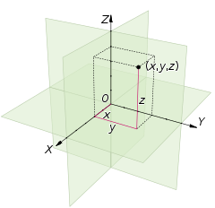
Координаты точки в прямоугольной системе координат в трехмерном пространстве
Определение точки М в трехмерном пространстве. Пусть имеются Mx, My, Mz, являющиеся проекциями точки М на соответствующие оси Ох, Оу, Оz. Тогда значения этих точек на осях Ох, Оу, Оz примут значения xM, yM, zM. Изобразим это на координатных прямых.

Чтобы получить проекции точки M, необходимо добавить перпендикулярные прямые Ох, Оу, Оz продолжить и изобразит в виде плоскостей, которые проходят через M. Таким образом, плоскости пересекутся в Mx, My, Mz

Каждая точка трехмерного пространства имеет свои данные (xM, yM, zM) , которые имеют название координаты точки M, , xM, yM, zM- это числа, называемые абсциссой, ординатой и аппликатой заданной точки M. Для данного суждения верно и обратное утверждение: каждая упорядоченная тройка действительных чисел (xM, yM, zM) в заданной прямоугольной системе координат имеет одну соответствующую точку M трехмерного пространства.
Система координат — комплекс определений, реализующий метод координат, то есть способ определять положение и перемещение точки или тела с помощью чисел или других символов. Совокупность чисел, определяющих положение конкретной точки, называется координатами этой точки. В математике координаты — совокупность чисел, сопоставленных точкам многообразия в некоторой карте определённого атласа.

Координаты на прямой
Если на прямой задано направление, то такую прямую называют направленной, а выбранное направление — положительным. Например, на горизонтальной прямой можно отметить направление вправо, тогда будем говорить, что направленная прямая имеет положительное направление вправо. Можно с таким же правом считать положительным и направление влево. Направление прямой будем указывать стрелкой (рис. 1).
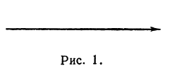
Выберем на направленной прямой точку, которую назовем началом отсчета или началом координат, и будем обозначать ее буквой О.
Кроме того, выберем отрезок, длину которого будем считать единицей длины. Этот отрезок назовем единицей масштаба.
Определение:
Прямая линия, на которой указаны: начало отсчета, единица масштаба и направление отсчета, называется осью координат.
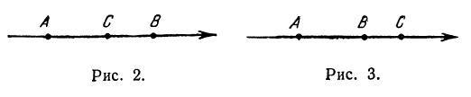
Рассмотрим отрезок, расположенный на оси координат. Если одну из точек, ограничивающих отрезок, назовем началом отрезка, а другую—его концом, то отрезок будем называть направленным отрезком. Направленный отрезок обозначают двумя буквами, например: АВ, СМ, КР, причем на первом месте ставят букву, обозначающую начало, на втором—букву, обозначающую конец. Таким образом, запись АВ показывает, что начало отрезка есть точка А, а конец — точка В. Направление отрезка считается от начала к концу.
Если направление отрезка совпадает с направлением оси, то отрезок называют положительно направленным; если же его направление противоположно направлению оси, то — отрицательно направленным. Таким образом, отрезки АВ и ВА имеют противоположные направления. Это записывают так:

Отметим, что положительный отрезок может находиться в любом месте координатной оси, только его направление должно совпадать с направлением оси.
Сложение направленных отрезков производится по следующему правилу:
Для того чтобы сложить два направленных отрезка, нужно к концу первого приложить начало второго; тогда отрезок, имеющий началом начало первого отрезка и концом конец второго, называют суммой двух направленных отрезков.
Из этого определения вытекает, что сумма отрезков АВ и ВС равна отрезку АС при любом расположении точек А, В, С, т. е. всегда:

(рис. 2 и 3).
Координатным отрезком точки А называется направленный отрезок, имеющий начало в точке О (т. е. в начале координат), а концом — рассматриваемую точку А.
Всякий направленный отрезок, лежащий на оси, можно выразить через координатные отрезки его начала и конца. В самом деле, рассмотрим направленный отрезок АВ. На основании равенства (2) можно написать

(здесь вместо точки В поставлена точка О, а вместо точки С точка В) или
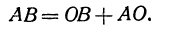
Отрезок ОВ есть координатный отрезок (его начало есть точка О), но отрезок АО не является координатным, поскольку его начало не является началом координат. Но в силу равенства (1)
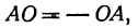
поэтому можно написать

Получен следующий результат:
Направленный отрезок равен разности координатного отрезка его конца и координатного отрезка его начала.
Это верно для любого отрезка, лежащего на координатной оси.
Теперь дадим одно из самых важных определений: Координатой точки на координатной оси называется число, равное по абсолютной величине длине координатного отрезка этой точки и по знаку совпадающее со знаком координатного отрезка.
Точку А, имеющую координатной число х, будем обозначать А (х).
Указанные на рис. 4 точки имеют следующие координаты:

Будем также писать
Если даны точки А(х1) и В(х2), то на основании формул (3) и (4) получим
т. е. направленный отрезок равен разности координат его конца и начала.
Отсюда сразу получаем, что длина отрезка равна абсолютной величине разности координат его конца и начала.
Длину отрезка будем обозначать, пользуясь знаком | |, т. е. знаком абсолютной величины. Таким образом, длина отрезка АВ будет записываться так:
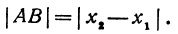
Пример:
Если даны точки А (+4), В (+8), то отрезок АВ = (+8) — (+4), а его длина |АВ|= |+ 4 | = 4.
Если даны точки М (+5) и Р (+3), то отрезок МР = (+3)—(+5) = —2, а его длина |МР| = | —2| = 2. Даны две точки: Q (+ 3) и S (—4). Длина отрезка
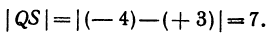
Даны две точки R (— 6) и Т (—2); отрезок RТ = ( — 2) — (—6) = +4, а его длина | RТ | = 4.
Пример:
Начало отрезка АВ находится в точке А (—950), а конец—в точке В ( —1200); найти его направление и длину.
Отрезок АВ = ( — 1200)—( — 950) = —250. Так как он
получился отрицательным, то его направление противоположно направлению оси. Его длина равна | АВ | = | —250 | = 250.
Задача:
На координатной оси даны две точки: A (x1) и В (x2) Найти точку С, лежащую между ними и делящую отрезок АВ в отношении т : п.
Чтобы найти точку, надо найти ее координату. По условию задачи должно быть
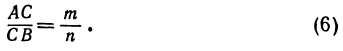
Обозначая координату искомой точки С через х и выражая отрезки через координаты, т. е. применяя формулу (5), получим, что АС = х—х1, СВ = х2 — х. Подставляя эти выражения в равенство (6), будем иметь
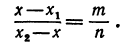
Решая последнее уравнение относительно х, найдем:
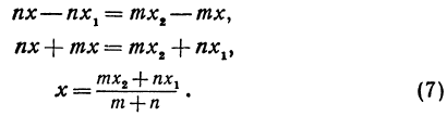
Это и есть координата искомой точки.
Пример:
Найти точку С, делящую отрезок АВ в отношении 1:2, если даны начало отрезка А (+ 3) и конец В ( + 5) (рис. 5).
Здесь т = 1, п = 2, х1=-3, х2 = 5. Применяя формулу (7), получим
Пример:
Найти точку М, делящую расстояние между точками Р ( — 2) и Q (—9) в отношении 3:4 (рис. 5). Здесь т = 3, п = 4, х1 = —2, х2 = —9. По формуле (7) находим
Если т = n т. е. точка С делит отрезок АВ пополам, тогда формула (7) перепишется так:
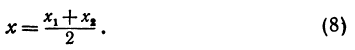
Таким образом, координата точки, делящей отрезок пополам, равна средней арифметической координат его начала и конца.
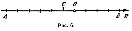
Пример:
Найдем середину отрезка, заключенного между точками А (—6) и B (4) (рис. 6).
Применяя формулу (8), получим, что
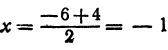
Координаты на плоскости
Возьмем на плоскости две взаимно перпендикулярные прямые, пересекающиеся в точке О. На каждой из этих прямых зададим направление, указав его стрелкой (рис. 7).
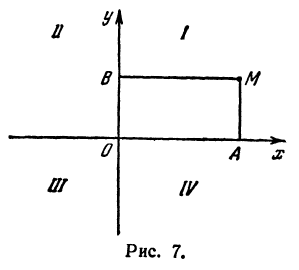
Установим масштаб, общий для обеих прямых, а за начало отсчета выберем точку О.
Определение:
Координатными осями на плоскости называются две взаимно перпендикулярные прямые, на которых установлены: 1) на-правления, 2) масштаб и 3) общая точка отсчета.
Назовем одну из осей осью Ох или осью абсцисс, другую — осью Оу или осью ординат. Точку их пересечения назовем началом координат.
Возьмем произвольную точку M, лежащую на плоскости, и опустим из нее перпендикуляры на оси координат, т. е. найдем ее проекции на оси. Обозначим проекцию на ось Ох через А, а проекцию на ось Оу через В. Обозначим координату точки А (по оси Ох) через х, а координату точки В (по оси Оу) через у. Введем определение:
Определение:
Абсциссой точки называется координата ее проекции на ось Ох. Ординатой точки называется координата ее проекции на ось Оу.
Абсциссу точки обычно обозначают буквой х, ординату— буквой у. Точку М, имеющую абсциссу х и ординату у, обозначают следующим образом: пишут скобку и в ней на первом месте ставят абсциссу, на втором ординату и разделяют эти два числа запятой или точкой с запятой. Таким образом, запись точки выглядит так: М(х, у).
Координатные оси разделяют плоскость на четыре части, которые называют четвертями.
Первой четвертью называется та часть плоскости, в которой абсцисса и ордината положительны.
Второй четвертью — та часть, в которой абсцисса отрицательна, а ордината положительна.
Третьей четвертью — та часть, в которой абсцисса и ордината отрицательны, и, наконец, четвертой, — та часть, в которой абсцисса положительна, а ордината отрицательна (рис. 7), На рис. 8 указаны точки M1 (5, 2), М2 ( — 1, 1), М3 (-1, -3), М4 (2, -3). Заметим, что абсцисса х = ОА по абсолютной величине равна расстоянию точки от оси ординат, так как ОА = ВМ (см. рис. 7), а ордината — расстоянию точки М от оси абсцисс, так как ОВ = АМ.
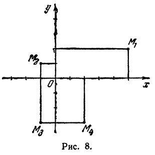
Пример:
Найти точку Р( — 4, 2) (рис. 9), Возьмем на оси Ох точку А с координатой —4, ее координатный отрезок ОА = —4. На оси Оу возьмем точку В с координатным отрезком ОВ= 2. Восставим перпендикуляры к осям из точек А и В, точка их пересечения и даст искомую точку Р.
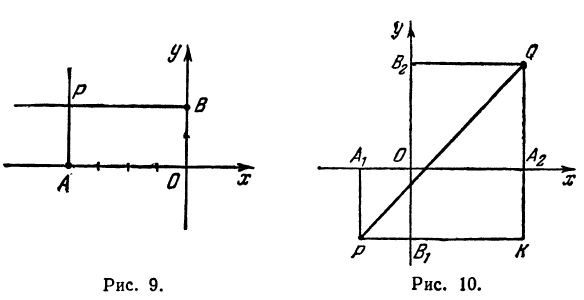
Задача:
Найти расстояние между точками Р (х1, у1) и Q( х1, у1 ). Иначе говоря, нужно найти длину отрезка РQ(рис. 10).
Обозначим проекцию точки Р на ось Ох через А1, а ее проекцию на ось Оу — через В1. Проекцию точки Q на ось Ох обозначим через А2 и через В2— ее проекцию на ось Oy. Тогда ОА1 = х1, ОВ1 = y1, ОА2 = х2, ОВ2 = у2. Из точки Р проведем прямую, параллельную оси Ох, до пересечения с прямой A2Q в точке К. Рассмотрим треугольник PKQ. По теореме Пифагора имеем
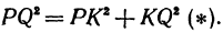
Но РК = А1А2, KQ = B1B2, как противоположные стороны прямоугольников; кроме того, на основании формулы (3 из § 1) направленные отрезки А1А2 и В1В2 будут равны

Подставляя полученные выражения в (*), получим
откуда

т. е. расстояние между двумя точками равно корню квадратному из суммы квадратов разностей координат.
Примечание:
Расстояние между двумя точками, так же как длина отрезка, всегда положительно, поэтому в формуле (1) перед квадратным корнем берут только знак плюс.
Пример:
Найти расстояние между точками Р (— 2, — 1) и Q (2, 2). Применяя формулу (1), получим

Пример:
Найти длину отрезка MN, если даны М (8, 2) и N(2, 10). Применяя формулу (1), получим

Задача:
Найти точку С, делящую отрезок PQ в отношении т : п, если известны координаты точек Р (х1, у1) и Q (х2, у2). По условию задачи надо найти такую точку С, чтобы было выполнено равенство

Решение:
Обозначим, как и выше, проекции точки Р на оси через А1 и В1, а проекции точки Q—через А2 и В2; тогда ОА1 = х1 , OB1 = y1, ОА2 =х2, ОВ2=у2 (рис. 11). Кроме того, обозначим координаты искомой точки С через х и у, а ее проекции на оси — через А и В, т. е. ОА = х, ОВ = у.
Так как прямые А1Р, АС и А2Q параллельны между собой, то на основании теоремы о пропорциональных отрезках можно записать, что
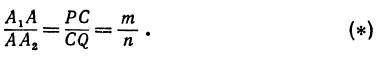
Но А1А = ОА — ОА1 = х—х1, АА2 = ОА2 — ОА = х2—х; поэтому, подставляя в равенство (*), будем иметь уравнение
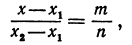
решая которое найдем абсциссу точки С:
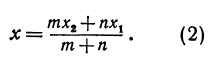
Рассуждая аналогично о проекциях на ось Оу, т. е. о точках В1, В и В2, получим ординату точки С, делящей отрезок в отношении т : п,
Итак, искомая точка С имеет координаты, определяемые равенствами (2) и (3).
Пример:
Найти точку, делящую в отношении 1:2 отрезок PQ, где Р (4, —3) и Q (8, 0). Здесь х1 = 4, у1 = — 3, х2 = 8, у2 = 0, т = 1, п = 2. Применяя формулы (2) и (3), получим:
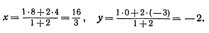
Пример:
Найти точку, делящую расстояние между точками А (4, 2) и B (8, 10) в отношении 3 : 1. Здесь х1=-4, у1 = 2, х2 = 8, у2= 10, т = 3, п = 1. По формулам (2) и (3) находим:
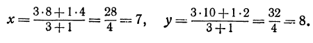
Следствие (из формул (2) и (3)). Если точка С делит отрезок РQ пополам, то т = n, поэтому
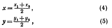
т. е. абсцисса середины отрезка равна средней арифметической абсцисс его начала и конца; ордината середины отрезка равна средней арифметической ординат его начала и конца.
Задача:
Даны три вершины треугольника: А (7, 0), В (4, 4) и С (7, 10). Найти длину биссектрисы угла A (рис. 12).
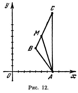
Найдем длины сторон АВ и АС. Для этого применим формулу (1):
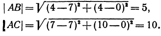
Обозначим точку пересечения биссектрисы угла А с противоположной стороной ВС через М, а ее координаты—через х и у. Помня, что биссектриса внутреннего угла треугольника делит противоположную сторону на отрезки, пропорциональные прилежащим сторонам, можно утверждать, что точка М делит отрезок ВС в отношении 5 : 10 =  ; поэтому, применяя формулы (2) и (3), получим:
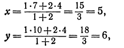
т. е. М (5, 6).
Теперь вычисляем длину биссектрисы между точками А(7, 0) и М(5, 6):

Задача:
Найти точку пересечения медиан треугольника, вершинами которого являются точки А(4, 6), В(—8, 10), С( —2, —6) (рис. 13).
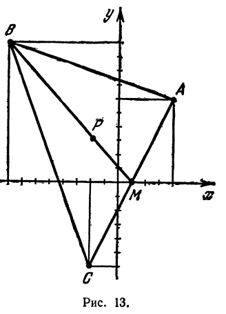
Точка пересечения медиан делит каждую из медиан в отношении 2:1, считая от вершины треугольника. Обозначим через М середину стороны АС; по формулам (4) и (5) можно найти ее координаты:
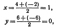
т. е. М(19 0). Точка Р пересечения медиан делит отрезок ВМ в отношении 2:1, поэтому ее координаты найдутся по формулам (2)
и (3):
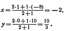
Итак, искомая точка
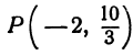
Задача:
Записать условие того, что точка М (х, у) находится на расстоянии По формуле (1) имеем

или, возводя обе части равенства в квадрат, получим

Это равенство есть уравнение с двумя неизвестными х и у. Этому уравнению удовлетворяют координаты любой точки, лежащей на расстоянии 5 от точки С. Иначе говоря, ему удовлетворяют координаты любой точки, принадлежащей геометрическому месту точек, расстояние которых от точки С равно 5. Это геометрическое место есть окружность.
Следовательно, можно сказать, что уравнение (*) есть уравнение окружности с центром в точке С и радиуса 5.
В следующих главах будут рассмотрены уравнения с двумя неизвестными х и у и те линии (геометрические места), точки которых имеют координаты, удовлетворяющие этим уравнениям.
Числовая ось
Числовой осью называют направленную прямую, на которой указывается начальная точка О и задается некоторый «эталон» длины Е. Каждой точке  этой прямой отвечает вещественное число, равное длине отрезка
  если расположено правее точки О, и равное этой
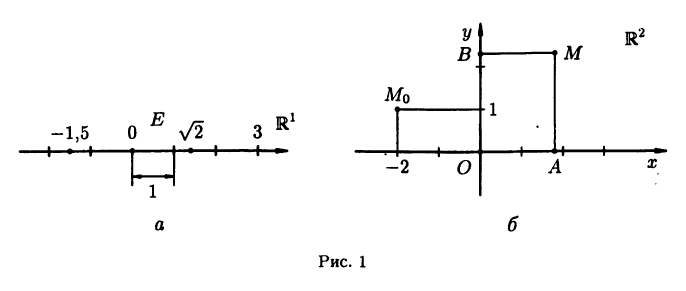
длине со знаком минус — в противном случае (см. рис. 1 а). Числовую ось будем обозначать  (смысл этого обозначения прояснится ниже).
Указанное соответствие между точками числовой оси и множеством вещественных чисел  является взаимно однозначным, т. е. каждой точке
  соответствует единственное число
  , обратно, каждому числу соответствует единственная точка Таким образом, множество . вещественных чисел можно отождествлять с числовой осью , чем мы будем впредь постоянно пользоваться.
Декартова система координат
Декартовой (прямоугольной) системой координат на плоскости называют две взаимно перпендикулярные числовые оси  и
и  , имеющие общее начало О и одинаковые единицы масштаба (см. рис. 1 б). Ось называют осью абсцисс, а ось — осью ординат. Плоскость
  называют координатной плоскостью и обозначают
Пусть М — произвольная точка координатной плоскости. Опустим из нее перпендикуляры МА и МВ на оси и соответственно. Декартовыми координатами точки М называют числа, которым соответствуют точки А к В. Например, точка  имеет декартовы координаты
 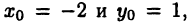 что записывается в виде
  Точка О имеет координаты (0,0).
Полярная система координат
В плоскости зададим луч — полярную ось, выходящий из точки О — полюса полярной системы координат (см. рис. 2 а). Произвольная точка М плоскости определяется парой чисел  называемой ее полярными координатами, где р — длина отрезка ОМ, а
  — выраженный в радианах угол между ОМ и осью . Угол в считается положительным, если откладывается против часовой стрелки, и отрицательным в противоположном случае. Точка О имеет полярные координаты
  где — любой угол.
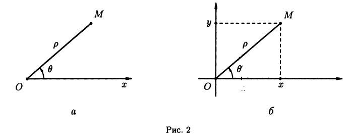
Полярные и декартовы координаты, заданные на одной плоскости (см. рис. 2 6), связаны очевидными равенствами:

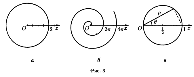
Полярные координаты удобны для задания многих кривых. Например, уравнение р=2 описывает окружность, изображенную на рис. За. Уравнение  описывает спираль Архимеда (рис . Уравнение
  описывает окружность с диаметром 1 и с центром в точке
  (рис. Зв).
Системы координат в пространстве
Декартова система координат в пространстве определяется тремя взаимно перпендикулярными осями , и  , называемыми соответственно осями абсцисс, ординат и аппликат (см. рис. 4 а). Проcтранство
  обозначают
  . Положение точки М в определяется тройкой чисел
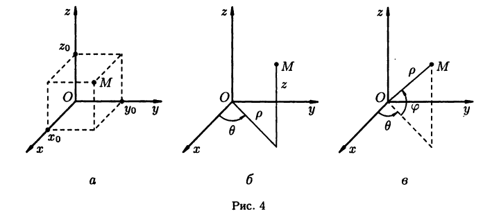
Аналогами полярной системы координат в пространстве служат цилиндрическая и сферическая системы координат.
Цилиндрическая система координат (рис. 4 б) представляет собой объединение полярной системы координат в плоскости с аппликатой z:

где 
Сферическая система координат (рис. 4 в) связана с декартовой системой равенствами
где 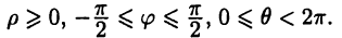
Пространство
Пространство 
На плоскости и в пространстве положение точки в декартовых координатах полностью определяется соответственно, парой и тройкой чисел вида [ ) и (x,y,z). Желая обобщить эти геометрические подходы, в анализе вводят понятие пространства
Упорядоченную систему из  вещественных чисел
 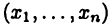 называют -мерной точкой, а множество всех -мерных точек называют —мерным пространством или короче — пространством .
Понятие пространства естественно дополнить понятиями основных операций над его элементами. По определению полагают
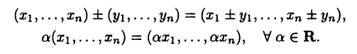
Наконец, обобщая известную из аналитической геометрии формулу, определяют расстояние между двумя точками 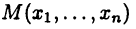 и
и 

Прямую, плоскость и пространство можно рассматривать как пространства ,  и соответственно. Ниже это будет практиковаться постоянно.
Решение заданий и задач по предметам:
- Математика
- Высшая математика
- Математический анализ
- Линейная алгебра
Дополнительные лекции по высшей математике:
- Тождественные преобразования алгебраических выражений
- Функции и графики
- Преобразования графиков функций
- Квадратная функция и её графики
- Алгебраические неравенства
- Неравенства
- Неравенства с переменными
- Прогрессии в математике
- Арифметическая прогрессия
- Геометрическая прогрессия
- Показатели в математике
- Логарифмы в математике
- Исследование уравнений
- Уравнения высших степеней
- Уравнения высших степеней с одним неизвестным
- Комплексные числа
- Непрерывная дробь (цепная дробь)
- Алгебраические уравнения
- Неопределенные уравнения
- Соединения
- Бином Ньютона
- Число е
- Непрерывные дроби
- Функция
- Исследование функций
- Предел
- Интеграл
- Двойной интеграл
- Тройной интеграл
- Интегрирование
- Неопределённый интеграл
- Определенный интеграл
- Криволинейные интегралы
- Поверхностные интегралы
- Несобственные интегралы
- Кратные интегралы
- Интегралы, зависящие от параметра
- Квадратный трехчлен
- Производная
- Применение производной к исследованию функций
- Приложения производной
- Дифференциал функции
- Дифференцирование в математике
- Формулы и правила дифференцирования
- Дифференциальное исчисление
- Дифференциальные уравнения
- Дифференциальные уравнения первого порядка
- Дифференциальные уравнения высших порядков
- Дифференциальные уравнения в частных производных
- Тригонометрические функции
- Тригонометрические уравнения и неравенства
- Показательная функция
- Показательные уравнения
- Обобщенная степень
- Взаимно обратные функции
- Логарифмическая функция
- Уравнения и неравенства
- Положительные и отрицательные числа
- Алгебраические выражения
- Иррациональные алгебраические выражения
- Преобразование алгебраических выражений
- Преобразование дробных алгебраических выражений
- Разложение многочленов на множители
- Многочлены от одного переменного
- Алгебраические дроби
- Пропорции
- Уравнения
- Системы уравнений
- Системы уравнений высших степеней
- Системы алгебраических уравнений
- Системы линейных уравнений
- Системы дифференциальных уравнений
- Арифметический квадратный корень
- Квадратные и кубические корни
- Извлечение квадратного корня
- Рациональные числа
- Иррациональные числа
- Арифметический корень
- Квадратные уравнения
- Иррациональные уравнения
- Последовательность
- Ряды сходящиеся и расходящиеся
- Тригонометрические функции произвольного угла
- Тригонометрические формулы
- Обратные тригонометрические функции
- Теорема Безу
- Математическая индукция
- Показатель степени
- Показательные функции и логарифмы
- Множество
- Множество действительных чисел
- Числовые множества
- Преобразование рациональных выражений
- Преобразование иррациональных выражений
- Геометрия
- Действительные числа
- Степени и корни
- Степень с рациональным показателем
- Тригонометрические функции угла
- Тригонометрические функции числового аргумента
- Тригонометрические выражения и их преобразования
- Преобразование тригонометрических выражений
- Комбинаторика
- Вычислительная математика
- Прямая линия на плоскости и ее уравнения
- Прямая и плоскость
- Линии и уравнения
- Прямая линия
- Уравнения прямой и плоскости в пространстве
- Кривые второго порядка
- Кривые и поверхности второго порядка
- Числовые ряды
- Степенные ряды
- Ряды Фурье
- Преобразование Фурье
- Функциональные ряды
- Функции многих переменных
- Метод координат
- Гармонический анализ
- Вещественные числа
- Предел последовательности
- Аналитическая геометрия
- Аналитическая геометрия на плоскости
- Аналитическая геометрия в пространстве
- Функции одной переменной
- Высшая алгебра
- Векторная алгебра
- Векторный анализ
- Векторы
- Скалярное произведение векторов
- Векторное произведение векторов
- Смешанное произведение векторов
- Операции над векторами
- Непрерывность функций
- Предел и непрерывность функций нескольких переменных
- Предел и непрерывность функции одной переменной
- Производные и дифференциалы функции одной переменной
- Частные производные и дифференцируемость функций нескольких переменных
- Дифференциальное исчисление функции одной переменной
- Матрицы
- Линейные и евклидовы пространства
- Линейные отображения
- Дифференциальные теоремы о среднем
- Теория устойчивости дифференциальных уравнений
- Функции комплексного переменного
- Преобразование Лапласа
- Теории поля
- Операционное исчисление
- Системы координат
- Рациональная функция
- Интегральное исчисление
- Интегральное исчисление функций одной переменной
- Дифференциальное исчисление функций нескольких переменных
- Отношение в математике
- Математическая логика
- Графы в математике
- Линейные пространства
- Первообразная и неопределенный интеграл
- Линейная функция
- Выпуклые множества точек

Координаты в математике
- Координаты в математике
-
— величины, определяющие положение точки. В Декартовых прямоугольных К. положение точки определяется тремя расстояниями ее от трех взаимно перпендикулярных плоскостей; пересечения этих плоскостей представляют собой три прямые, выходящие из одной точки, называемой началом, и именуются осями К. Декартовы косые К. — в них три координатные плоскости составляют между собой углы не прямые, и за К. точки принимаются расстояния ее от плоскостей, считаемые по прямым параллельным осям. Однородные К — положение точки определяется величинами X, Y, Z, T, помноженными на произвольные множители, причем сами эти величины представляют собой расстояния точки от четырех сторон некоторого тетраэдра. Между величинами Х, Y, Z и Т всегда существует соотношение вида aX+bY+cZ+dT =1, где а, b, с, d есть константы. Каждая Декартова К. x может быть выражена формулой x=(тХ+пТ+pZ+qT)/(аХ+bY+cZ+dT) и все уравнения выходят однородными. Трилинейные К. В геометрии на плоскости вместо тетраэдра берется треугольник и положение точки определяется расстояниями ее от сторон этого треугольника, помноженными на произвольные множители. Бинарные К. — за К. точки, на определенной прямой, могут быть приняты расстояния точки от двух данных точек, помноженные на произвольные множители. За полярные К. на плоскости принимаются: расстояние ОМ = ρ точки М от определенной точки О, называемой началом, и угол θ, составляемый прямой ОМ с некоторой определенной прямой ОА, называемой полярной осью. Расстояние ОМ = ρ называется радиусом-вектором. Чтобы от этих К. перейти к полярным К. в пространстве, представим себе, что плоскость, проходящая через точку M и полярную ось ОА, вращается около полярной оси, и введем новую К. λ = угол, составляемый этой плоскостью с некоторой неподвижной плоскостью, проходящей через ОА.
Координаты сферические. — Если начало полярных координат взять в центре сферы, то все точки сфер имеют одинаковый радиус-вектор и останутся изменяемыми только углы θ и λ. Обычно вместо θ берется другая координата φ =90- θ, которая называется широтой, угол же λ — долготой. Этими двумя координатами определяются географические положения точек земного шара. В координатах полуполярных или цилиндрических положение точки определяется расстоянием ее от некоторой плоскости и полярными координатами ρ и θ ее проекции на эту плоскость. В биполярных координатах на плоскости положение точки определяется расстояниями ее от двух данных точек. Тангенциальные координаты — положение плоскости может быть определено тремя величинами, например, тремя отрезками, отсекаемыми плоскостью от трех данных прямых, выходящих из одной точки. Уравнением f (u, v, w)=O между этими отрезками u, v, w определяется множество плоскостей, огибающих некоторую поверхность. Если это уравнение линейное, то им определяется точка и величины u, v, w называются тангенциальными координатами. Полярные тангенциальные координаты — Гальфен называет длину р перпендикуляра, опущенного из неподвижной точки на касательную к кривой, и угол θ, составляемый этим перпендикуляром с данным направлением, полярными тангенциальными координатами. Плюкеровы координаты прямой: прямая в Декартовых координатах выражается уравнениями: bz—cy+a’=0; cx—az+b’=O, из которых вытекает: ay—bx+c’=O, при условии aa’+bb’+cc’=O. Величины: a, a’, b, b’, c, c’ определяют положение прямой и называются координатами прямой. Криволинейные координаты — если три поверхности f1(х, у, z)= λ, f2(х, у, z)= μ, f3(х, у, z)= ν, в которых λ, μ и ν есть произвольные параметры, пересекаются в точке, положение которой определяется, то параметры λ, μ и ν могут быть приняты за координаты этой точки. С изменением параметров каждое из написанных трех уравнений представляет особое семейство координатных поверхностей. Если за координатные поверхности приняты эллипсоиды, однополые гиперболоиды и двуполые гиперболоиды, представляющие собой поверхности конфокальные, то координаты называются эллиптическими.
Н. Делоне.
Энциклопедический словарь Ф.А. Брокгауза и И.А. Ефрона. — С.-Пб.: Брокгауз-Ефрон.
1890—1907.
Полезное
Смотреть что такое «Координаты в математике» в других словарях:
-
КООРДИНАТЫ (в математике) — КООРДИНАТЫ (от лат. co совместно и ordinatus упорядоченный, определенный), числа, заданием которых определяется положение точки на плоскости, на поверхности или в пространстве. Прямоугольные (декартовы) координаты точки на плоскости суть… … Энциклопедический словарь
-
Координаты, в математике — величины, определяющие положение точки. В Декартовых прямоугольных К. положение точки определяется тремя расстояниями ее от трех взаимно перпендикулярных плоскостей; пересечения этих плоскостей представляют собой три прямые, выходящие из одной… … Энциклопедический словарь Ф.А. Брокгауза и И.А. Ефрона
-
Координаты в астрономии — величины, посредством которых определяют положение небесных светил, относительно некоторых прилично избранных плоскостей, линий и точек. Так, относя положение светила к местному горизонту, употребляют высоту и азимут; относя к плоскости небесного … Энциклопедический словарь Ф.А. Брокгауза и И.А. Ефрона
-
Координаты астрономические — величины, посредством которых определяют положение небесных светил, относительно некоторых прилично избранных плоскостей, линий и точек. Так, относя положение светила к местному горизонту, употребляют высоту и азимут; относя к плоскости небесного … Энциклопедический словарь Ф.А. Брокгауза и И.А. Ефрона
-
КООРДИНАТЫ — (ср. век. лат., от лат. cum с, и ordinare приводить в порядок). В аналит. геометрии: такие величины, которые служат для определения положения какой нибудь точки. Словарь иностранных слов, вошедших в состав русского языка. Чудинов А.Н., 1910.… … Словарь иностранных слов русского языка
-
КООРДИНАТЫ — (от лат. со – совместно и ordinatus – упорядоченный) осн. моменты, определяющие данность. В математике – величины, определяющие положение точки; часто наглядно они изображаются с помощью отрезков. Если отходящие от точки (начало координат) прямые … Философская энциклопедия
-
Координаты вектора — ― коэффициенты единственно возможной линейной комбинации базисных векторов в выбранной системе координат, равной данному вектору. где координаты вектора. Свойства Равные векторы в единой системе координат имеют равные координаты Координаты … Википедия
-
Координаты — (от лат. со совместно + ordinatus упорядоченный) 1) в широком смысле основные моменты, определяющие данность; 2) (в математике) числа, заданием которых определяется положение точки на прямой, на плоскости или в пространстве; так, в декартовых… … Начала современного естествознания
-
прямоугольные координаты — см. Координаты. * * * ПРЯМОУГОЛЬНЫЕ КООРДИНАТЫ ПРЯМОУГОЛЬНЫЕ КООРДИНАТЫ, см. Координаты (см. КООРДИНАТЫ (в математике)) … Энциклопедический словарь
-
Цилиндрические координаты — см. соотв. статью (Координаты, в математике) … Энциклопедический словарь Ф.А. Брокгауза и И.А. Ефрона
Во многих ситуациях реальной жизни мы используем два числа (или другие символы), чтобы точно описать нужный нам объект.
Место в зрительном зале задаётся номером ряда и номером кресла в ряду.

Рис. (1). Зрительный зал, схема
На шахматной доске позиция шахматной фигуры задаётся названием столбца и номером ряда.

Рис. (2). Шахматная доска
Любая карта (или глобус) разделена на квадраты, и, подобно шахматной доске, каждый квадрат задаётся двумя номерами.

Рис. (3). Географическая карта
На экране компьютера каждая точка задаётся двумя номерами.

Рис. (4). Пиксельная сетка экрана

Рис. (5). Рене Декарт
Французский философ и математик Рене Декарт ((1596)–(1650)) уже в XVII веке предложил метод двух координат для нахождения точки на плоскости. Поэтому система координат названа его именем.
Декартовую систему координат образуют:
1. две перпендикулярные прямые, на которых указано направление возрастания чисел. Горизонтальная прямая называется осью Ox, или осью абсцисс. Вертикальная прямая называется осью Oy, или осью ординат.
2. Точка пересечения прямых — начало координатной системы, она часто обозначается через букву O.
3. Отрезки на каждой оси длиной в одну единицу измерения.

Рис. (6). Система координат
Для любой точки находят две координаты (x) и (y) (абсциссу и ординату) и записывают как AxA;yA.
На рисунке показаны координаты A2;4, то есть абсцисса точки (A) равна (2), а ордината точки (A) равна (4).
Если на плоскости выбрана система координат, то такую плоскость называют координатной плоскостью.
Так как оси координат делят плоскость на (4) части, каждая из них имеет номер и называется квадрантом.
В I квадранте находится положительная часть оси абсцисс и оси ординат.
Во II квадранте находится положительная часть оси ординат и отрицательная часть оси абсцисс.
В III квадранте находится отрицательная часть оси абсцисс и оси ординат.
В IV квадранте находится положительная часть оси абсцисс и отрицательная часть оси ординат.

Рис. (7). Система координат, квадранты
Источники:
Рис. 1. Зрительный зал, схема. © Якласс
Рис. 2. Шахматная доска. Указание авторства не требуется, 2021.06.03, бесплатно для коммерческого использования, https://pixabay.com/images/id-3791454/
Рис. 3. Географическая карта. Указание авторства не требуется, 2021.06.03, бесплатно для коммерческого использования, https://pixabay.com/images/id-1149538/
Рис. 4. Пиксельная сетка экрана. © Якласс
Рис. 5. Рене Декарт. Общественное достояние. 2021.06.03, https://clck.ru/Nhumi
Рис. 6. Система координат. © Якласс
Рис. 7. Система координат, квадранты. © Якласс
Справочник ОГЭ по математике. Раздел 6. Координаты на прямой и плоскости.
На ОГЭ по математике по данному разделу необходимо знать:
- понятие о координатах, точки на прямой и на плоскости;
- определение основных видов числовых промежутков;
- формулы координат середины отрезка, расстояния между точками;
- уравнение прямой;
- уравнение окружности;
- уравнения и неравенства с двумя переменными.
На ОГЭ по математике по данному разделу необходимо уметь:
- объяснять и иллюстрировать понятие координатной прямой, модуля числа и декартовой системы координат;
- использовать формулы координат середины отрезка, расстояния между точками, уравнения прямой и окружности для решения задач;
- использовать координатный метод для задач на вычисление;
- строить графики уравнений и неравенств с двумя переменными.
ОГЛАВЛЕНИЕ Перейти в другие разделы: 5.1. …
6. Координаты на прямой и плоскости
6.1. Координатная прямая.
6.1.1. Изображение чисел точками координатной прямой.
6.1.2. Геометрический смысл модуля.
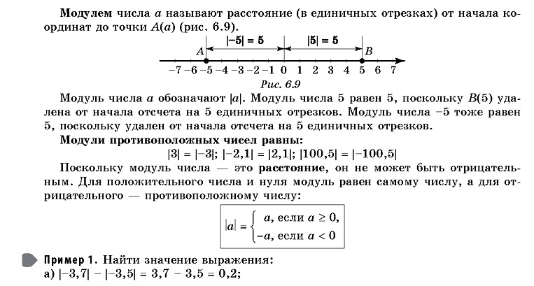
6.1.3. Числовые промежутки: интервал, отрезок, луч.
6.2. Декартовы координаты на плоскости.
6.2.1. Декартовы координаты на плоскости. Координаты точки.
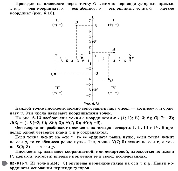
6.2.2. Координаты середины отрезка.
6.2.3. Формула расстояния между двумя точками плоскости.
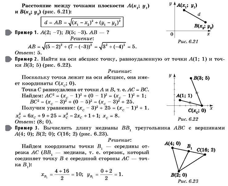
6.2.4. Уравнение прямой, угловой коэффициент прямой, условие параллельности прямых.
6.2.5. Уравнение окружности.
6.2.6. Графическая интерпретация уравнений с двумя переменными и их систем.
6.2.7. Графическая интерпретация неравенств с двумя переменными и их систем.
Вы смотрели конспект по математике «6. Координаты на прямой и плоскости (справочник ОГЭ)»:
- 6.1. Координатная прямая.
- 6.1.1. Изображение чисел точками координатной прямой.
- 6.1.2. Геометрический смысл модуля.
- 6.1.3. Числовые промежутки: интервал, отрезок, луч.
- 6.2. Декартовы координаты на плоскости.
- 6.2.1. Декартовы координаты на плоскости. Координаты точки.
- 6.2.2. Координаты середины отрезка.
- 6.2.3. Формула расстояния между двумя точками плоскости.
- 6.2.4. Уравнение прямой, угловой коэффициент прямой, условие параллельности прямых.
- 6.2.5. Уравнение окружности.
- 6.2.6. Графическая интерпретация уравнений с двумя переменными и их систем.
- 6.2.7. Графическая интерпретация неравенств с двумя переменными и их систем.
Выберите дальнейшее действие:
-
Перейти в Кодификатор ОГЭ по математике
-
Перейти к Оглавлению Справочника ОГЭ по математике (Третьяк И.В.)
-
Купить Справочник ОГЭ по математике (Третьяк И.В.)